Select Expression
Select Expression
Syntax Definition
A selection expression (selectExpr) is a component of a SELECT clause, each selectExpr corresponds to a column in the query result set, and its syntax is defined as follows:
selectClause
    : SELECT resultColumn (',' resultColumn)*
    ;

resultColumn
    : selectExpr (AS alias)?
    ;

selectExpr
    : '(' selectExpr ')'
    | '-' selectExpr
    | selectExpr ('*' | '/' | '%') selectExpr
    | selectExpr ('+' | '-') selectExpr
    | functionName '(' selectExpr (',' selectExpr)* functionAttribute* ')'
    | timeSeriesSuffixPath
    | number
    ;
From this syntax definition, selectExpr can contain:
- suffix of time series path
- function
- Built-in aggregation functions, see Aggregate Query for details.
- Time series generation function
- User-defined functions, see UDF for details.
- expressions
- Arithmetic operation expressions
- Time series generating nested expressions
- Aggregate query nested expressions
- Numeric constants (could be used in expressions only)
Arithmetic Query
Please note that Aligned Timeseries has not been supported in Arithmetic Query yet. An error message is expected if you use Arithmetic Query with Aligned Timeseries selected.
Operators
Unary Arithmetic Operators
Supported operators: +, -
Supported input data types: INT32, INT64, FLOAT and DOUBLE
Output data type: consistent with the input data type
Binary Arithmetic Operators
Supported operators: +, -, *, /, %
Supported input data types: INT32, INT64, FLOAT and DOUBLE
Output data type: DOUBLE
Note: Only when the left operand and the right operand under a certain timestamp are not null, the binary arithmetic operation will have an output value.
Example
select s1, - s1, s2, + s2, s1 + s2, s1 - s2, s1 * s2, s1 / s2, s1 % s2 from root.sg.d1Result:
+-----------------------------+-------------+--------------+-------------+-------------+-----------------------------+-----------------------------+-----------------------------+-----------------------------+-----------------------------+
|                         Time|root.sg.d1.s1|-root.sg.d1.s1|root.sg.d1.s2|root.sg.d1.s2|root.sg.d1.s1 + root.sg.d1.s2|root.sg.d1.s1 - root.sg.d1.s2|root.sg.d1.s1 * root.sg.d1.s2|root.sg.d1.s1 / root.sg.d1.s2|root.sg.d1.s1 % root.sg.d1.s2|
+-----------------------------+-------------+--------------+-------------+-------------+-----------------------------+-----------------------------+-----------------------------+-----------------------------+-----------------------------+
|1970-01-01T08:00:00.001+08:00|          1.0|          -1.0|          1.0|          1.0|                          2.0|                          0.0|                          1.0|                          1.0|                          0.0|
|1970-01-01T08:00:00.002+08:00|          2.0|          -2.0|          2.0|          2.0|                          4.0|                          0.0|                          4.0|                          1.0|                          0.0|
|1970-01-01T08:00:00.003+08:00|          3.0|          -3.0|          3.0|          3.0|                          6.0|                          0.0|                          9.0|                          1.0|                          0.0|
|1970-01-01T08:00:00.004+08:00|          4.0|          -4.0|          4.0|          4.0|                          8.0|                          0.0|                         16.0|                          1.0|                          0.0|
|1970-01-01T08:00:00.005+08:00|          5.0|          -5.0|          5.0|          5.0|                         10.0|                          0.0|                         25.0|                          1.0|                          0.0|
+-----------------------------+-------------+--------------+-------------+-------------+-----------------------------+-----------------------------+-----------------------------+-----------------------------+-----------------------------+
Total line number = 5
It costs 0.014s
Time Series Generating Functions
The time series generating function takes several time series as input and outputs one time series. Unlike the aggregation function, the result set of the time series generating function has a timestamp column.
All time series generating functions can accept * as input.
IoTDB supports hybrid queries of time series generating function queries and raw data queries.
Please note that Aligned Timeseries has not been supported in queries with hybrid functions yet. An error message is expected if you use hybrid functions with Aligned Timeseries selected in a query statement.
Mathematical Functions
Currently, IoTDB supports the following mathematical functions. The behavior of these mathematical functions is consistent with the behavior of these functions in the Java Math standard library.
| Function Name | Allowed Input Series Data Types | Output Series Data Type | Corresponding Implementation in the Java Standard Library |
|---|---|---|---|
| SIN | INT32 / INT64 / FLOAT / DOUBLE | DOUBLE | Math#sin(double) |
| COS | INT32 / INT64 / FLOAT / DOUBLE | DOUBLE | Math#cos(double) |
| TAN | INT32 / INT64 / FLOAT / DOUBLE | DOUBLE | Math#tan(double) |
| ASIN | INT32 / INT64 / FLOAT / DOUBLE | DOUBLE | Math#asin(double) |
| ACOS | INT32 / INT64 / FLOAT / DOUBLE | DOUBLE | Math#acos(double) |
| ATAN | INT32 / INT64 / FLOAT / DOUBLE | DOUBLE | Math#atan(double) |
| SINH | INT32 / INT64 / FLOAT / DOUBLE | DOUBLE | Math#sinh(double) |
| COSH | INT32 / INT64 / FLOAT / DOUBLE | DOUBLE | Math#cosh(double) |
| TANH | INT32 / INT64 / FLOAT / DOUBLE | DOUBLE | Math#tanh(double) |
| DEGREES | INT32 / INT64 / FLOAT / DOUBLE | DOUBLE | Math#toDegrees(double) |
| RADIANS | INT32 / INT64 / FLOAT / DOUBLE | DOUBLE | Math#toRadians(double) |
| ABS | INT32 / INT64 / FLOAT / DOUBLE | Same type as the input series | Math#abs(int) / Math#abs(long) /Math#abs(float) /Math#abs(double) |
| SIGN | INT32 / INT64 / FLOAT / DOUBLE | DOUBLE | Math#signum(double) |
| CEIL | INT32 / INT64 / FLOAT / DOUBLE | DOUBLE | Math#ceil(double) |
| FLOOR | INT32 / INT64 / FLOAT / DOUBLE | DOUBLE | Math#floor(double) |
| ROUND | INT32 / INT64 / FLOAT / DOUBLE | DOUBLE | Math#rint(double) |
| EXP | INT32 / INT64 / FLOAT / DOUBLE | DOUBLE | Math#exp(double) |
| LN | INT32 / INT64 / FLOAT / DOUBLE | DOUBLE | Math#log(double) |
| LOG10 | INT32 / INT64 / FLOAT / DOUBLE | DOUBLE | Math#log10(double) |
| SQRT | INT32 / INT64 / FLOAT / DOUBLE | DOUBLE | Math#sqrt(double) |
Example:
select s1, sin(s1), cos(s1), tan(s1) from root.sg1.d1 limit 5 offset 1000;Result:
+-----------------------------+-------------------+-------------------+--------------------+-------------------+
|                         Time|     root.sg1.d1.s1|sin(root.sg1.d1.s1)| cos(root.sg1.d1.s1)|tan(root.sg1.d1.s1)|
+-----------------------------+-------------------+-------------------+--------------------+-------------------+
|2020-12-10T17:11:49.037+08:00|7360723084922759782| 0.8133527237573284|  0.5817708713544664| 1.3980636773094157|
|2020-12-10T17:11:49.038+08:00|4377791063319964531|-0.8938962705202537|  0.4482738644511651| -1.994085181866842|
|2020-12-10T17:11:49.039+08:00|7972485567734642915| 0.9627757585308978|-0.27030138509681073|-3.5618602479083545|
|2020-12-10T17:11:49.040+08:00|2508858212791964081|-0.6073417341629443| -0.7944406950452296| 0.7644897069734913|
|2020-12-10T17:11:49.041+08:00|2817297431185141819|-0.8419358900502509| -0.5395775727782725| 1.5603611649667768|
+-----------------------------+-------------------+-------------------+--------------------+-------------------+
Total line number = 5
It costs 0.008s
String Processing Functions
Currently, IoTDB supports the following string processing functions:
| Function Name | Allowed Input Series Data Types | Required Attributes | Output Series Data Type | Description |
|---|---|---|---|---|
| STRING_CONTAINS | TEXT | s: the sequence to search for | BOOLEAN | Determine whether s is in the string |
| STRING_MATCHES | TEXT | regex: the regular expression to which the string is to be matched | BOOLEAN | Determine whether the string can be matched by regex |
Example:
select s1, string_contains(s1, 's'='warn'), string_matches(s1, 'regex'='[^\\s]+37229') from root.sg1.d4;Result:
+-----------------------------+--------------+-------------------------------------------+------------------------------------------------------+
|                         Time|root.sg1.d4.s1|string_contains(root.sg1.d4.s1, "s"="warn")|string_matches(root.sg1.d4.s1, "regex"="[^\\s]+37229")|
+-----------------------------+--------------+-------------------------------------------+------------------------------------------------------+
|1970-01-01T08:00:00.001+08:00|    warn:-8721|                                       true|                                                 false|
|1970-01-01T08:00:00.002+08:00|  error:-37229|                                      false|                                                  true|
|1970-01-01T08:00:00.003+08:00|     warn:1731|                                       true|                                                 false|
+-----------------------------+--------------+-------------------------------------------+------------------------------------------------------+
Total line number = 3
It costs 0.007s
Selector Functions
Currently, IoTDB supports the following selector functions:
| Function Name | Allowed Input Series Data Types | Required Attributes | Output Series Data Type | Description |
|---|---|---|---|---|
| TOP_K | INT32 / INT64 / FLOAT / DOUBLE / TEXT | k: the maximum number of selected data points, must be greater than 0 and less than or equal to 1000 | Same type as the input series | Returns k data points with the largest values in a time series. |
| BOTTOM_K | INT32 / INT64 / FLOAT / DOUBLE / TEXT | k: the maximum number of selected data points, must be greater than 0 and less than or equal to 1000 | Same type as the input series | Returns k data points with the smallest values in a time series. |
Example:
select s1, top_k(s1, 'k'='2'), bottom_k(s1, 'k'='2') from root.sg1.d2 where time > 2020-12-10T20:36:15.530+08:00;Result:
+-----------------------------+--------------------+------------------------------+---------------------------------+
|                         Time|      root.sg1.d2.s1|top_k(root.sg1.d2.s1, "k"="2")|bottom_k(root.sg1.d2.s1, "k"="2")|
+-----------------------------+--------------------+------------------------------+---------------------------------+
|2020-12-10T20:36:15.531+08:00| 1531604122307244742|           1531604122307244742|                             null|
|2020-12-10T20:36:15.532+08:00|-7426070874923281101|                          null|                             null|
|2020-12-10T20:36:15.533+08:00|-7162825364312197604|          -7162825364312197604|                             null|
|2020-12-10T20:36:15.534+08:00|-8581625725655917595|                          null|             -8581625725655917595|
|2020-12-10T20:36:15.535+08:00|-7667364751255535391|                          null|             -7667364751255535391|
+-----------------------------+--------------------+------------------------------+---------------------------------+
Total line number = 5
It costs 0.006s
Variation Trend Calculation Functions
Currently, IoTDB supports the following variation trend calculation functions:
| Function Name | Allowed Input Series Data Types | Output Series Data Type | Description |
|---|---|---|---|
| TIME_DIFFERENCE | INT32 / INT64 / FLOAT / DOUBLE / BOOLEAN / TEXT | INT64 | Calculates the difference between the time stamp of a data point and the time stamp of the previous data point. There is no corresponding output for the first data point. |
| DIFFERENCE | INT32 / INT64 / FLOAT / DOUBLE | Same type as the input series | Calculates the difference between the value of a data point and the value of the previous data point. There is no corresponding output for the first data point. |
| NON_NEGATIVE_DIFFERENCE | INT32 / INT64 / FLOAT / DOUBLE | Same type as the input series | Calculates the absolute value of the difference between the value of a data point and the value of the previous data point. There is no corresponding output for the first data point. |
| DERIVATIVE | INT32 / INT64 / FLOAT / DOUBLE | DOUBLE | Calculates the rate of change of a data point compared to the previous data point, the result is equals to DIFFERENCE / TIME_DIFFERENCE. There is no corresponding output for the first data point. |
| NON_NEGATIVE_DERIVATIVE | INT32 / INT64 / FLOAT / DOUBLE | DOUBLE | Calculates the absolute value of the rate of change of a data point compared to the previous data point, the result is equals to NON_NEGATIVE_DIFFERENCE / TIME_DIFFERENCE. There is no corresponding output for the first data point. |
Example:
select s1, time_difference(s1), difference(s1), non_negative_difference(s1), derivative(s1), non_negative_derivative(s1) from root.sg1.d1 limit 5 offset 1000;Result:
+-----------------------------+-------------------+-------------------------------+--------------------------+---------------------------------------+--------------------------+---------------------------------------+
|                         Time|     root.sg1.d1.s1|time_difference(root.sg1.d1.s1)|difference(root.sg1.d1.s1)|non_negative_difference(root.sg1.d1.s1)|derivative(root.sg1.d1.s1)|non_negative_derivative(root.sg1.d1.s1)|
+-----------------------------+-------------------+-------------------------------+--------------------------+---------------------------------------+--------------------------+---------------------------------------+
|2020-12-10T17:11:49.037+08:00|7360723084922759782|                              1|      -8431715764844238876|                    8431715764844238876|    -8.4317157648442388E18|                  8.4317157648442388E18|
|2020-12-10T17:11:49.038+08:00|4377791063319964531|                              1|      -2982932021602795251|                    2982932021602795251|     -2.982932021602795E18|                   2.982932021602795E18|
|2020-12-10T17:11:49.039+08:00|7972485567734642915|                              1|       3594694504414678384|                    3594694504414678384|     3.5946945044146785E18|                  3.5946945044146785E18|
|2020-12-10T17:11:49.040+08:00|2508858212791964081|                              1|      -5463627354942678834|                    5463627354942678834|     -5.463627354942679E18|                   5.463627354942679E18|
|2020-12-10T17:11:49.041+08:00|2817297431185141819|                              1|        308439218393177738|                     308439218393177738|     3.0843921839317773E17|                  3.0843921839317773E17|
+-----------------------------+-------------------+-------------------------------+--------------------------+---------------------------------------+--------------------------+---------------------------------------+
Total line number = 5
It costs 0.014s
Constant Timeseries Generating Functions
The constant timeseries generating function is used to generate a timeseries in which the values of all data points are the same.
The constant timeseries generating function accepts one or more timeseries inputs, and the timestamp set of the output data points is the union of the timestamp sets of the input timeseries.
Currently, IoTDB supports the following constant timeseries generating functions:
| Function Name | Required Attributes | Output Series Data Type | Description |
|---|---|---|---|
| CONST | value: the value of the output data point type: the type of the output data point, it can only be INT32 / INT64 / FLOAT / DOUBLE / BOOLEAN / TEXT | Determined by the required attribute type | Output the user-specified constant timeseries according to the attributes value and type. |
| PI | None | DOUBLE | Data point value: a double value of π, the ratio of the circumference of a circle to its diameter, which is equals to Math.PI in the Java Standard Library. |
| E | None | DOUBLE | Data point value: a double value of e, the base of the natural logarithms, which is equals to Math.E in the Java Standard Library. |
Example:
select s1, s2, const(s1, 'value'='1024', 'type'='INT64'), pi(s2), e(s1, s2) from root.sg1.d1;Result:
select s1, s2, const(s1, 'value'='1024', 'type'='INT64'), pi(s2), e(s1, s2) from root.sg1.d1;
+-----------------------------+--------------+--------------+-----------------------------------------------------+------------------+---------------------------------+
|                         Time|root.sg1.d1.s1|root.sg1.d1.s2|const(root.sg1.d1.s1, "value"="1024", "type"="INT64")|pi(root.sg1.d1.s2)|e(root.sg1.d1.s1, root.sg1.d1.s2)|
+-----------------------------+--------------+--------------+-----------------------------------------------------+------------------+---------------------------------+
|1970-01-01T08:00:00.000+08:00|           0.0|           0.0|                                                 1024| 3.141592653589793|                2.718281828459045|
|1970-01-01T08:00:00.001+08:00|           1.0|          null|                                                 1024|              null|                2.718281828459045|
|1970-01-01T08:00:00.002+08:00|           2.0|          null|                                                 1024|              null|                2.718281828459045|
|1970-01-01T08:00:00.003+08:00|          null|           3.0|                                                 null| 3.141592653589793|                2.718281828459045|
|1970-01-01T08:00:00.004+08:00|          null|           4.0|                                                 null| 3.141592653589793|                2.718281828459045|
+-----------------------------+--------------+--------------+-----------------------------------------------------+------------------+---------------------------------+
Total line number = 5
It costs 0.005s
Data Type Conversion Function
The IoTDB currently supports 6 data types, including INT32, INT64 ,FLOAT, DOUBLE, BOOLEAN, TEXT. When we query or evaluate data, we may need to convert data types, such as TEXT to INT32, or improve the accuracy of the data, such as FLOAT to DOUBLE. Therefore, IoTDB supports the use of cast functions to convert data types.
| Function Name | Required Attributes | Output Series Data Type | Series Data Type Description |
|---|---|---|---|
| CAST | type: the type of the output data point, it can only be INT32 / INT64 / FLOAT / DOUBLE / BOOLEAN / TEXT | Determined by the required attribute type | Converts data to the type specified by the type argument. |
Notes
- The value of type BOOLEAN is
true, when data is converted to BOOLEAN if INT32 and INT64 are not 0, FLOAT and DOUBLE are not 0.0, TEXT is not empty string or "false", otherwisefalse.
IoTDB> show timeseries root.sg.d1.*;
+-------------+-----+-------------+--------+--------+-----------+----+----------+
|   timeseries|alias|storage group|dataType|encoding|compression|tags|attributes|
+-------------+-----+-------------+--------+--------+-----------+----+----------+
|root.sg.d1.s3| null|      root.sg|   FLOAT|     RLE|     SNAPPY|null|      null|
|root.sg.d1.s4| null|      root.sg|  DOUBLE|     RLE|     SNAPPY|null|      null|
|root.sg.d1.s5| null|      root.sg|    TEXT|   PLAIN|     SNAPPY|null|      null|
|root.sg.d1.s6| null|      root.sg| BOOLEAN|     RLE|     SNAPPY|null|      null|
|root.sg.d1.s1| null|      root.sg|   INT32|     RLE|     SNAPPY|null|      null|
|root.sg.d1.s2| null|      root.sg|   INT64|     RLE|     SNAPPY|null|      null|
+-------------+-----+-------------+--------+--------+-----------+----+----------+
Total line number = 6
It costs 0.006s
IoTDB> select * from root.sg.d1;
+-----------------------------+-------------+-------------+-------------+-------------+-------------+-------------+
|                         Time|root.sg.d1.s3|root.sg.d1.s4|root.sg.d1.s5|root.sg.d1.s6|root.sg.d1.s1|root.sg.d1.s2|
+-----------------------------+-------------+-------------+-------------+-------------+-------------+-------------+
|1970-01-01T08:00:00.001+08:00|          1.1|          1.1|         test|        false|            1|            1|
|1970-01-01T08:00:00.002+08:00|         -2.2|         -2.2|        false|         true|           -2|           -2|
|1970-01-01T08:00:00.003+08:00|          0.0|          0.0|         true|         true|            0|            0|
+-----------------------------+-------------+-------------+-------------+-------------+-------------+-------------+
Total line number = 3
It costs 0.009s

IoTDB> select cast(s1, 'type'='BOOLEAN'), cast(s2, 'type'='BOOLEAN'), cast(s3, 'type'='BOOLEAN'), cast(s4, 'type'='BOOLEAN'), cast(s5, 'type'='BOOLEAN') from root.sg.d1;
+-----------------------------+-------------------------------------+-------------------------------------+-------------------------------------+-------------------------------------+-------------------------------------+
|                         Time|cast(root.sg.d1.s1, "type"="BOOLEAN")|cast(root.sg.d1.s2, "type"="BOOLEAN")|cast(root.sg.d1.s3, "type"="BOOLEAN")|cast(root.sg.d1.s4, "type"="BOOLEAN")|cast(root.sg.d1.s5, "type"="BOOLEAN")|
+-----------------------------+-------------------------------------+-------------------------------------+-------------------------------------+-------------------------------------+-------------------------------------+
|1970-01-01T08:00:00.001+08:00|                                 true|                                 true|                                 true|                                 true|                                 true|
|1970-01-01T08:00:00.002+08:00|                                 true|                                 true|                                 true|                                 true|                                false|
|1970-01-01T08:00:00.003+08:00|                                false|                                false|                                false|                                false|                                 true|
+-----------------------------+-------------------------------------+-------------------------------------+-------------------------------------+-------------------------------------+-------------------------------------+
Total line number = 3
It costs 0.012s- The value of type INT32, INT64, FLOAT, DOUBLE are 1 or 1.0 and TEXT is "true", when BOOLEAN data is true, otherwise 0, 0.0 or "false".
IoTDB> select cast(s6, 'type'='INT32'), cast(s6, 'type'='INT64'), cast(s6, 'type'='FLOAT'), cast(s6, 'type'='DOUBLE'), cast(s6, 'type'='TEXT') from root.sg.d1;
+-----------------------------+-----------------------------------+-----------------------------------+-----------------------------------+------------------------------------+----------------------------------+
|                         Time|cast(root.sg.d1.s6, "type"="INT32")|cast(root.sg.d1.s6, "type"="INT64")|cast(root.sg.d1.s6, "type"="FLOAT")|cast(root.sg.d1.s6, "type"="DOUBLE")|cast(root.sg.d1.s6, "type"="TEXT")|
+-----------------------------+-----------------------------------+-----------------------------------+-----------------------------------+------------------------------------+----------------------------------+
|1970-01-01T08:00:00.001+08:00|                                  0|                                  0|                                0.0|                                 0.0|                             false|
|1970-01-01T08:00:00.002+08:00|                                  1|                                  1|                                1.0|                                 1.0|                              true|
|1970-01-01T08:00:00.003+08:00|                                  1|                                  1|                                1.0|                                 1.0|                              true|
+-----------------------------+-----------------------------------+-----------------------------------+-----------------------------------+------------------------------------+----------------------------------+
Total line number = 3
It costs 0.016s- When TEXT is converted to INT32, INT64, or FLOAT, the TEXT is first converted to DOUBLE and then to the corresponding type, which may cause loss of precision. It will skip directly if the data can not be converted.
IoTDB> select cast(s5, 'type'='INT32'), cast(s5, 'type'='INT64'), cast(s5, 'type'='FLOAT') from root.sg.d1;
+----+-----------------------------------+-----------------------------------+-----------------------------------+
|Time|cast(root.sg.d1.s5, "type"="INT32")|cast(root.sg.d1.s5, "type"="INT64")|cast(root.sg.d1.s5, "type"="FLOAT")|
+----+-----------------------------------+-----------------------------------+-----------------------------------+
+----+-----------------------------------+-----------------------------------+-----------------------------------+
Empty set.
It costs 0.009s
Example
Example data:
IoTDB> select text from root.test;
+-----------------------------+--------------+
|                         Time|root.test.text|
+-----------------------------+--------------+
|1970-01-01T08:00:00.001+08:00|           1.1|
|1970-01-01T08:00:00.002+08:00|             1|
|1970-01-01T08:00:00.003+08:00|   hello world|
|1970-01-01T08:00:00.004+08:00|         false|
+-----------------------------+--------------+
SQL:
select cast(text, 'type'='BOOLEAN'), cast(text, 'type'='INT32'), cast(text, 'type'='INT64'), cast(text, 'type'='FLOAT'), cast(text, 'type'='DOUBLE') from root.test;Result:
+-----------------------------+--------------------------------------+------------------------------------+------------------------------------+------------------------------------+-------------------------------------+
|                         Time|cast(root.test.text, "type"="BOOLEAN")|cast(root.test.text, "type"="INT32")|cast(root.test.text, "type"="INT64")|cast(root.test.text, "type"="FLOAT")|cast(root.test.text, "type"="DOUBLE")|
+-----------------------------+--------------------------------------+------------------------------------+------------------------------------+------------------------------------+-------------------------------------+
|1970-01-01T08:00:00.001+08:00|                                  true|                                   1|                                   1|                                 1.1|                                  1.1|
|1970-01-01T08:00:00.002+08:00|                                  true|                                   1|                                   1|                                 1.0|                                  1.0|
|1970-01-01T08:00:00.003+08:00|                                  true|                                null|                                null|                                null|                                 null|
|1970-01-01T08:00:00.004+08:00|                                 false|                                null|                                null|                                null|                                 null|
+-----------------------------+--------------------------------------+------------------------------------+------------------------------------+------------------------------------+-------------------------------------+
Total line number = 4
It costs 0.078s
Condition Functions
Condition functions are used to check whether timeseries data points satisfy some specific condition.
They return BOOLEANs.
Currently, IoTDB supports the following condition functions:
| Function Name | Allowed Input Series Data Types | Required Attributes | Output Series Data Type | Series Data Type Description |
|---|---|---|---|---|
| ON_OFF | INT32 / INT64 / FLOAT / DOUBLE | threshold: a double type variate | BOOLEAN | Return ts_value >= threshold. |
| IN_RANGR | INT32 / INT64 / FLOAT / DOUBLE | lower: DOUBLE typeupper: DOUBLE type | BOOLEAN | Return ts_value >= lower && value <= upper. |
Example Data:
IoTDB> select ts from root.test;
+-----------------------------+------------+
|                         Time|root.test.ts|
+-----------------------------+------------+
|1970-01-01T08:00:00.001+08:00|           1|
|1970-01-01T08:00:00.002+08:00|           2|
|1970-01-01T08:00:00.003+08:00|           3|
|1970-01-01T08:00:00.004+08:00|           4|
+-----------------------------+------------+
Example 1
SQL:
select ts, on_off(ts, 'threshold'='2') from root.test;Output:
IoTDB> select ts, on_off(ts, 'threshold'='2') from root.test;
+-----------------------------+------------+-------------------------------------+
|                         Time|root.test.ts|on_off(root.test.ts, "threshold"="2")|
+-----------------------------+------------+-------------------------------------+
|1970-01-01T08:00:00.001+08:00|           1|                                false|
|1970-01-01T08:00:00.002+08:00|           2|                                 true|
|1970-01-01T08:00:00.003+08:00|           3|                                 true|
|1970-01-01T08:00:00.004+08:00|           4|                                 true|
+-----------------------------+------------+-------------------------------------+
Example 2
Sql:
select ts, in_range(ts, 'lower'='2', 'upper'='3.1') from root.test;Output:
IoTDB> select ts, in_range(ts,'lower'='2', 'upper'='3.1') from root.test;
+-----------------------------+------------+--------------------------------------------------+
|                         Time|root.test.ts|in_range(root.test.ts, "lower"="2", "upper"="3.1")|
+-----------------------------+------------+--------------------------------------------------+
|1970-01-01T08:00:00.001+08:00|           1|                                             false|
|1970-01-01T08:00:00.002+08:00|           2|                                              true|
|1970-01-01T08:00:00.003+08:00|           3|                                              true|
|1970-01-01T08:00:00.004+08:00|           4|                                             false|
+-----------------------------+------------+--------------------------------------------------+
Continuous Interval Functions
The continuous interval functions are used to query all continuous intervals that meet specified conditions.
They can be divided into two categories according to return value:
- Returns the start timestamp and time span of the continuous interval that meets the conditions (a time span of 0 means that only the start time point meets the conditions)
- Returns the start timestamp of the continuous interval that meets the condition and the number of points in the interval (a number of 1 means that only the start time point meets the conditions)
| Function Name | Input TSDatatype | Parameters | Output TSDatatype | Function Description |
|---|---|---|---|---|
| ZERO_DURATION | INT32/ INT64/ FLOAT/ DOUBLE/ BOOLEAN | min:Optional with default value 0Lmax:Optional with default value Long.MAX_VALUE | Long | Return intervals' start times and duration times in which the value is always 0(false), and the duration time t satisfy t >= min && t <= max. The unit of t is ms |
| NON_ZERO_DURATION | INT32/ INT64/ FLOAT/ DOUBLE/ BOOLEAN | min:Optional with default value 0Lmax:Optional with default value Long.MAX_VALUE | Long | Return intervals' start times and duration times in which the value is always not 0, and the duration time t satisfy t >= min && t <= max. The unit of t is ms |
| ZERO_COUNT | INT32/ INT64/ FLOAT/ DOUBLE/ BOOLEAN | min:Optional with default value 1Lmax:Optional with default value Long.MAX_VALUE | Long | Return intervals' start times and the number of data points in the interval in which the value is always 0(false). Data points number n satisfy n >= min && n <= max |
| NON_ZERO_COUNT | INT32/ INT64/ FLOAT/ DOUBLE/ BOOLEAN | min:Optional with default value 1Lmax:Optional with default value Long.MAX_VALUE | Long | Return intervals' start times and the number of data points in the interval in which the value is always not 0(false). Data points number n satisfy n >= min && n <= max |
Example
Example data:
IoTDB> select s1,s2,s3,s4,s5 from root.sg.d2;
+-----------------------------+-------------+-------------+-------------+-------------+-------------+
|                         Time|root.sg.d2.s1|root.sg.d2.s2|root.sg.d2.s3|root.sg.d2.s4|root.sg.d2.s5|
+-----------------------------+-------------+-------------+-------------+-------------+-------------+
|1970-01-01T08:00:00.000+08:00|            0|            0|          0.0|          0.0|        false|
|1970-01-01T08:00:00.001+08:00|            1|            1|          1.0|          1.0|         true|
|1970-01-01T08:00:00.002+08:00|            1|            1|          1.0|          1.0|         true|
|1970-01-01T08:00:00.003+08:00|            0|            0|          0.0|          0.0|        false|
|1970-01-01T08:00:00.004+08:00|            1|            1|          1.0|          1.0|         true|
|1970-01-01T08:00:00.005+08:00|            0|            0|          0.0|          0.0|        false|
|1970-01-01T08:00:00.006+08:00|            0|            0|          0.0|          0.0|        false|
|1970-01-01T08:00:00.007+08:00|            1|            1|          1.0|          1.0|         true|
+-----------------------------+-------------+-------------+-------------+-------------+-------------+
Sql:
select s1, zero_count(s1), non_zero_count(s2), zero_duration(s3), non_zero_duration(s4) from root.sg.d2;Result:
+-----------------------------+-------------+-------------------------+-----------------------------+----------------------------+--------------------------------+
|                         Time|root.sg.d2.s1|zero_count(root.sg.d2.s1)|non_zero_count(root.sg.d2.s2)|zero_duration(root.sg.d2.s3)|non_zero_duration(root.sg.d2.s4)|
+-----------------------------+-------------+-------------------------+-----------------------------+----------------------------+--------------------------------+
|1970-01-01T08:00:00.000+08:00|            0|                        1|                         null|                           0|                            null|
|1970-01-01T08:00:00.001+08:00|            1|                     null|                            2|                        null|                               1|
|1970-01-01T08:00:00.002+08:00|            1|                     null|                         null|                        null|                            null|
|1970-01-01T08:00:00.003+08:00|            0|                        1|                         null|                           0|                            null|
|1970-01-01T08:00:00.004+08:00|            1|                     null|                            1|                        null|                               0|
|1970-01-01T08:00:00.005+08:00|            0|                        2|                         null|                           1|                            null|
|1970-01-01T08:00:00.006+08:00|            0|                     null|                         null|                        null|                            null|
|1970-01-01T08:00:00.007+08:00|            1|                     null|                            1|                        null|                               0|
+-----------------------------+-------------+-------------------------+-----------------------------+----------------------------+--------------------------------+
Equal Size Bucket Sample Function
This function samples the input sequence in equal size buckets. That is, according to the downsampling ratio and downsampling method given by the user, the input sequence is equally divided into several buckets according to a fixed number of points, and sampled by the given sampling method within each bucket.
proportion: sample ratio, the value range is(0, 1].- four sampling methods:
equal_size_bucket_random_sampleequal_size_bucket_agg_sampleequal_size_bucket_m4_sampleequal_size_bucket_outlier_sample
Equal Size Bucket Random Sample
Random sampling is performed on the equally divided buckets.
| Function Name | Allowed Input Series Data Types | Required Attributes | Output Series Data Type | Series Data Type Description |
|---|---|---|---|---|
| EQUAL_SIZE_BUCKET_RANDOM_SAMPLE | INT32 / INT64 / FLOAT / DOUBLE | proportion The value range is (0, 1], the default is 0.1 | INT32 / INT64 / FLOAT / DOUBLE | Returns a random sample of equal buckets that matches the sampling ratio |
Example
Example data: root.ln.wf01.wt01.temperature has a total of 100 ordered data from 0.0-99.0.
IoTDB> select temperature from root.ln.wf01.wt01;
+-----------------------------+-----------------------------+
|                         Time|root.ln.wf01.wt01.temperature|
+-----------------------------+-----------------------------+
|1970-01-01T08:00:00.000+08:00|                          0.0|
|1970-01-01T08:00:00.001+08:00|                          1.0|
|1970-01-01T08:00:00.002+08:00|                          2.0|
|1970-01-01T08:00:00.003+08:00|                          3.0|
|1970-01-01T08:00:00.004+08:00|                          4.0|
|1970-01-01T08:00:00.005+08:00|                          5.0|
|1970-01-01T08:00:00.006+08:00|                          6.0|
|1970-01-01T08:00:00.007+08:00|                          7.0|
|1970-01-01T08:00:00.008+08:00|                          8.0|
|1970-01-01T08:00:00.009+08:00|                          9.0|
|1970-01-01T08:00:00.010+08:00|                         10.0|
|1970-01-01T08:00:00.011+08:00|                         11.0|
|1970-01-01T08:00:00.012+08:00|                         12.0|
|.............................|.............................|
|1970-01-01T08:00:00.089+08:00|                         89.0|
|1970-01-01T08:00:00.090+08:00|                         90.0|
|1970-01-01T08:00:00.091+08:00|                         91.0|
|1970-01-01T08:00:00.092+08:00|                         92.0|
|1970-01-01T08:00:00.093+08:00|                         93.0|
|1970-01-01T08:00:00.094+08:00|                         94.0|
|1970-01-01T08:00:00.095+08:00|                         95.0|
|1970-01-01T08:00:00.096+08:00|                         96.0|
|1970-01-01T08:00:00.097+08:00|                         97.0|
|1970-01-01T08:00:00.098+08:00|                         98.0|
|1970-01-01T08:00:00.099+08:00|                         99.0|
+-----------------------------+-----------------------------+
Sql:
select equal_size_bucket_random_sample(temperature,'proportion'='0.1') as random_sample from root.ln.wf01.wt01;Result:
+-----------------------------+-------------+
|                         Time|random_sample|
+-----------------------------+-------------+
|1970-01-01T08:00:00.007+08:00|          7.0|
|1970-01-01T08:00:00.014+08:00|         14.0|
|1970-01-01T08:00:00.020+08:00|         20.0|
|1970-01-01T08:00:00.035+08:00|         35.0|
|1970-01-01T08:00:00.047+08:00|         47.0|
|1970-01-01T08:00:00.059+08:00|         59.0|
|1970-01-01T08:00:00.063+08:00|         63.0|
|1970-01-01T08:00:00.079+08:00|         79.0|
|1970-01-01T08:00:00.086+08:00|         86.0|
|1970-01-01T08:00:00.096+08:00|         96.0|
+-----------------------------+-------------+
Total line number = 10
It costs 0.024s
Equal Size Bucket Aggregation Sample
The input sequence is sampled by the aggregation sampling method, and the user needs to provide an additional aggregation function parameter, namely
type: Aggregate type, which can beavgormaxorminorsumorextremeorvariance. By default,avgis used.extremerepresents the value with the largest absolute value in the equal bucket.variancerepresents the variance in the sampling equal buckets.
The timestamp of the sampling output of each bucket is the timestamp of the first point of the bucket.
| Function Name | Allowed Input Series Data Types | Required Attributes | Output Series Data Type | Series Data Type Description |
|---|---|---|---|---|
| EQUAL_SIZE_BUCKET_AGG_SAMPLE | INT32 / INT64 / FLOAT / DOUBLE | proportion The value range is (0, 1], the default is 0.1type: The value types are avg, max, min, sum, extreme, variance, the default is avg | INT32 / INT64 / FLOAT / DOUBLE | Returns equal bucket aggregation samples that match the sampling ratio |
Example
Example data: root.ln.wf01.wt01.temperature has a total of 100 ordered data from 0.0-99.0, and the test data is randomly sampled in equal buckets.
Sql:
select equal_size_bucket_agg_sample(temperature, 'type'='avg','proportion'='0.1') as agg_avg, equal_size_bucket_agg_sample(temperature, 'type'='max','proportion'='0.1') as agg_max, equal_size_bucket_agg_sample(temperature,'type'='min','proportion'='0.1') as agg_min, equal_size_bucket_agg_sample(temperature, 'type'='sum','proportion'='0.1') as agg_sum, equal_size_bucket_agg_sample(temperature, 'type'='extreme','proportion'='0.1') as agg_extreme, equal_size_bucket_agg_sample(temperature, 'type'='variance','proportion'='0.1') as agg_variance from root.ln.wf01.wt01;Result:
+-----------------------------+-----------------+-------+-------+-------+-----------+------------+
|                         Time|          agg_avg|agg_max|agg_min|agg_sum|agg_extreme|agg_variance|
+-----------------------------+-----------------+-------+-------+-------+-----------+------------+
|1970-01-01T08:00:00.000+08:00|              4.5|    9.0|    0.0|   45.0|        9.0|        8.25|
|1970-01-01T08:00:00.010+08:00|             14.5|   19.0|   10.0|  145.0|       19.0|        8.25|
|1970-01-01T08:00:00.020+08:00|             24.5|   29.0|   20.0|  245.0|       29.0|        8.25|
|1970-01-01T08:00:00.030+08:00|             34.5|   39.0|   30.0|  345.0|       39.0|        8.25|
|1970-01-01T08:00:00.040+08:00|             44.5|   49.0|   40.0|  445.0|       49.0|        8.25|
|1970-01-01T08:00:00.050+08:00|             54.5|   59.0|   50.0|  545.0|       59.0|        8.25|
|1970-01-01T08:00:00.060+08:00|             64.5|   69.0|   60.0|  645.0|       69.0|        8.25|
|1970-01-01T08:00:00.070+08:00|74.50000000000001|   79.0|   70.0|  745.0|       79.0|        8.25|
|1970-01-01T08:00:00.080+08:00|             84.5|   89.0|   80.0|  845.0|       89.0|        8.25|
|1970-01-01T08:00:00.090+08:00|             94.5|   99.0|   90.0|  945.0|       99.0|        8.25|
+-----------------------------+-----------------+-------+-------+-------+-----------+------------+
Total line number = 10
It costs 0.044s
Equal Size Bucket M4 Sample
The input sequence is sampled using the M4 sampling method. That is to sample the head, tail, min and max values for each bucket.
| Function Name | Allowed Input Series Data Types | Required Attributes | Output Series Data Type | Series Data Type Description |
|---|---|---|---|---|
| EQUAL_SIZE_BUCKET_M4_SAMPLE | INT32 / INT64 / FLOAT / DOUBLE | proportion The value range is (0, 1], the default is 0.1 | INT32 / INT64 / FLOAT / DOUBLE | Returns equal bucket M4 samples that match the sampling ratio |
Example
Example data: root.ln.wf01.wt01.temperature has a total of 100 ordered data from 0.0-99.0, and the test data is randomly sampled in equal buckets.
Sql:
select equal_size_bucket_m4_sample(temperature, 'proportion'='0.1') as M4_sample from root.ln.wf01.wt01;Result:
+-----------------------------+---------+
|                         Time|M4_sample|
+-----------------------------+---------+
|1970-01-01T08:00:00.000+08:00|      0.0|
|1970-01-01T08:00:00.001+08:00|      1.0|
|1970-01-01T08:00:00.038+08:00|     38.0|
|1970-01-01T08:00:00.039+08:00|     39.0|
|1970-01-01T08:00:00.040+08:00|     40.0|
|1970-01-01T08:00:00.041+08:00|     41.0|
|1970-01-01T08:00:00.078+08:00|     78.0|
|1970-01-01T08:00:00.079+08:00|     79.0|
|1970-01-01T08:00:00.080+08:00|     80.0|
|1970-01-01T08:00:00.081+08:00|     81.0|
|1970-01-01T08:00:00.098+08:00|     98.0|
|1970-01-01T08:00:00.099+08:00|     99.0|
+-----------------------------+---------+
Total line number = 12
It costs 0.065s
Equal Size Bucket Outlier Sample
This function samples the input sequence with equal number of bucket outliers, that is, according to the downsampling ratio given by the user and the number of samples in the bucket, the input sequence is divided into several buckets according to a fixed number of points. Sampling by the given outlier sampling method within each bucket.
| Function Name | Allowed Input Series Data Types | Required Attributes | Output Series Data Type | Series Data Type Description |
|---|---|---|---|---|
| EQUAL_SIZE_BUCKET_OUTLIER_SAMPLE | INT32 / INT64 / FLOAT / DOUBLE | The value range of proportion is (0, 1], the default is 0.1The value of type is avg or stendis or cos or prenextdis, the default is avg The value of number should be greater than 0, the default is 3 | INT32 / INT64 / FLOAT / DOUBLE | Returns outlier samples in equal buckets that match the sampling ratio and the number of samples in the bucket |
Parameter Description
proportion: sampling rationumber: the number of samples in each bucket, default3type: outlier sampling method, the value isavg: Take the average of the data points in the bucket, and find thetop numberfarthest from the average according to the sampling ratiostendis: Take the vertical distance between each data point in the bucket and the first and last data points of the bucket to form a straight line, and according to the sampling ratio, find thetop numberwith the largest distancecos: Set a data point in the bucket as b, the data point on the left of b as a, and the data point on the right of b as c, then take the cosine value of the angle between the ab and bc vectors. The larger the angle, the more likely it is an outlier. Find thetop numberwith the smallest cos valueprenextdis: Let a data point in the bucket be b, the data point to the left of b is a, and the data point to the right of b is c, then take the sum of the lengths of ab and bc as the yardstick, the larger the sum, the more likely it is to be an outlier, and find thetop numberwith the largest sum value
Example
Example data: root.ln.wf01.wt01.temperature has a total of 100 ordered data from 0.0-99.0. Among them, in order to add outliers, we make the number modulo 5 equal to 0 increment by 100.
IoTDB> select temperature from root.ln.wf01.wt01;
+-----------------------------+-----------------------------+
|                         Time|root.ln.wf01.wt01.temperature|
+-----------------------------+-----------------------------+
|1970-01-01T08:00:00.000+08:00|                          0.0|
|1970-01-01T08:00:00.001+08:00|                          1.0|
|1970-01-01T08:00:00.002+08:00|                          2.0|
|1970-01-01T08:00:00.003+08:00|                          3.0|
|1970-01-01T08:00:00.004+08:00|                          4.0|
|1970-01-01T08:00:00.005+08:00|                        105.0|
|1970-01-01T08:00:00.006+08:00|                          6.0|
|1970-01-01T08:00:00.007+08:00|                          7.0|
|1970-01-01T08:00:00.008+08:00|                          8.0|
|1970-01-01T08:00:00.009+08:00|                          9.0|
|1970-01-01T08:00:00.010+08:00|                         10.0|
|1970-01-01T08:00:00.011+08:00|                         11.0|
|1970-01-01T08:00:00.012+08:00|                         12.0|
|1970-01-01T08:00:00.013+08:00|                         13.0|
|1970-01-01T08:00:00.014+08:00|                         14.0|
|1970-01-01T08:00:00.015+08:00|                        115.0|
|1970-01-01T08:00:00.016+08:00|                         16.0|
|.............................|.............................|
|1970-01-01T08:00:00.092+08:00|                         92.0|
|1970-01-01T08:00:00.093+08:00|                         93.0|
|1970-01-01T08:00:00.094+08:00|                         94.0|
|1970-01-01T08:00:00.095+08:00|                        195.0|
|1970-01-01T08:00:00.096+08:00|                         96.0|
|1970-01-01T08:00:00.097+08:00|                         97.0|
|1970-01-01T08:00:00.098+08:00|                         98.0|
|1970-01-01T08:00:00.099+08:00|                         99.0|
+-----------------------------+-----------------------------+
Sql:
select equal_size_bucket_outlier_sample(temperature, 'proportion'='0.1', 'type'='avg', 'number'='2') as outlier_avg_sample, equal_size_bucket_outlier_sample(temperature, 'proportion'='0.1', 'type'='stendis', 'number'='2') as outlier_stendis_sample, equal_size_bucket_outlier_sample(temperature, 'proportion'='0.1', 'type'='cos', 'number'='2') as outlier_cos_sample, equal_size_bucket_outlier_sample(temperature, 'proportion'='0.1', 'type'='prenextdis', 'number'='2') as outlier_prenextdis_sample from root.ln.wf01.wt01;Result:
+-----------------------------+------------------+----------------------+------------------+-------------------------+
|                         Time|outlier_avg_sample|outlier_stendis_sample|outlier_cos_sample|outlier_prenextdis_sample|
+-----------------------------+------------------+----------------------+------------------+-------------------------+
|1970-01-01T08:00:00.005+08:00|             105.0|                 105.0|             105.0|                    105.0|
|1970-01-01T08:00:00.015+08:00|             115.0|                 115.0|             115.0|                    115.0|
|1970-01-01T08:00:00.025+08:00|             125.0|                 125.0|             125.0|                    125.0|
|1970-01-01T08:00:00.035+08:00|             135.0|                 135.0|             135.0|                    135.0|
|1970-01-01T08:00:00.045+08:00|             145.0|                 145.0|             145.0|                    145.0|
|1970-01-01T08:00:00.055+08:00|             155.0|                 155.0|             155.0|                    155.0|
|1970-01-01T08:00:00.065+08:00|             165.0|                 165.0|             165.0|                    165.0|
|1970-01-01T08:00:00.075+08:00|             175.0|                 175.0|             175.0|                    175.0|
|1970-01-01T08:00:00.085+08:00|             185.0|                 185.0|             185.0|                    185.0|
|1970-01-01T08:00:00.095+08:00|             195.0|                 195.0|             195.0|                    195.0|
+-----------------------------+------------------+----------------------+------------------+-------------------------+
Total line number = 10
It costs 0.041s
M4 Function
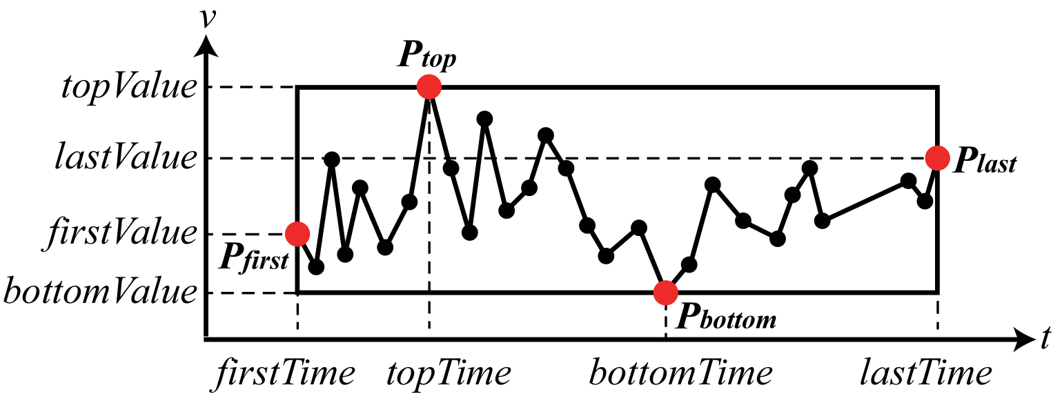
M4 is used to sample the first, last, bottom, top points for each sliding window:
- the first point is the point with the minimal time;
- the last point is the point with the maximal time;
- the bottom point is the point with the minimal value (if there are multiple such points, M4 returns one of them);
- the top point is the point with the maximal value (if there are multiple such points, M4 returns one of them).
| Function Name | Allowed Input Series Data Types | Attributes | Output Series Data Type | Series Data Type Description |
|---|---|---|---|---|
| M4 | INT32 / INT64 / FLOAT / DOUBLE | Different attributes used by the size window and the time window. The size window uses attributes windowSize and slidingStep. The time window uses attributes timeInterval, slidingStep, displayWindowBegin, and displayWindowEnd. More details see below. | INT32 / INT64 / FLOAT / DOUBLE | Returns the first, last, bottom, top points in each sliding window. M4 sorts and deduplicates the aggregated points within the window before outputting them. |
Attributes
(1) Attributes for the size window:
windowSize: The number of points in a window. Int data type. Required.slidingStep: Slide a window by the number of points. Int data type. Optional. If not set, default to the same aswindowSize.
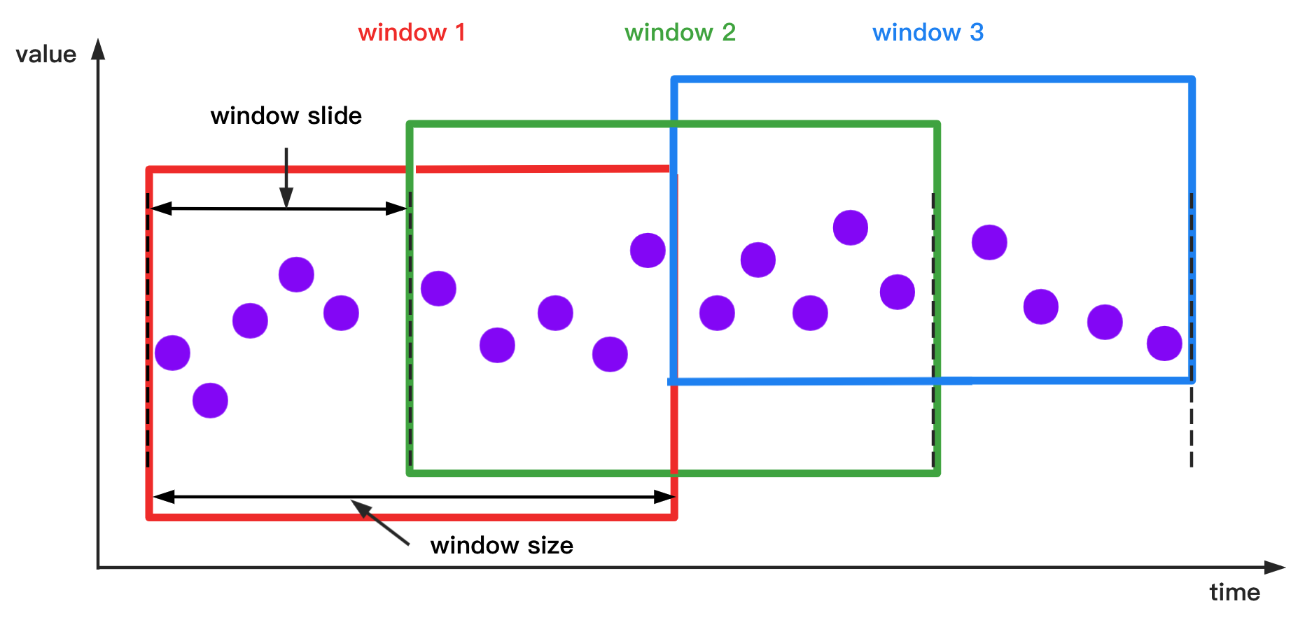
(2) Attributes for the time window:
timeInterval: The time interval length of a window. Long data type. Required.slidingStep: Slide a window by the time length. Long data type. Optional. If not set, default to the same astimeInterval.displayWindowBegin: The starting position of the window (included). Long data type. Optional. If not set, default to Long.MIN_VALUE, meaning using the time of the first data point of the input time series as the starting position of the window.displayWindowEnd: End time limit (excluded, essentially playing the same role asWHERE time < displayWindowEnd). Long data type. Optional. If not set, default to Long.MAX_VALUE, meaning there is no additional end time limit other than the end of the input time series itself.
Examples
Input series:
+-----------------------------+------------------+
|                         Time|root.vehicle.d1.s1|
+-----------------------------+------------------+
|1970-01-01T08:00:00.001+08:00|               5.0|
|1970-01-01T08:00:00.002+08:00|              15.0|
|1970-01-01T08:00:00.005+08:00|              10.0|
|1970-01-01T08:00:00.008+08:00|               8.0|
|1970-01-01T08:00:00.010+08:00|              30.0|
|1970-01-01T08:00:00.020+08:00|              20.0|
|1970-01-01T08:00:00.025+08:00|               8.0|
|1970-01-01T08:00:00.027+08:00|              20.0|
|1970-01-01T08:00:00.030+08:00|              40.0|
|1970-01-01T08:00:00.033+08:00|               9.0|
|1970-01-01T08:00:00.035+08:00|              10.0|
|1970-01-01T08:00:00.040+08:00|              20.0|
|1970-01-01T08:00:00.045+08:00|              30.0|
|1970-01-01T08:00:00.052+08:00|               8.0|
|1970-01-01T08:00:00.054+08:00|              18.0|
+-----------------------------+------------------+
SQL for query1:
select M4(s1,'timeInterval'='25','displayWindowBegin'='0','displayWindowEnd'='100') from root.vehicle.d1Output1:
+-----------------------------+-----------------------------------------------------------------------------------------------+
|                         Time|M4(root.vehicle.d1.s1, "timeInterval"="25", "displayWindowBegin"="0", "displayWindowEnd"="100")|
+-----------------------------+-----------------------------------------------------------------------------------------------+
|1970-01-01T08:00:00.001+08:00|                                                                                            5.0|
|1970-01-01T08:00:00.010+08:00|                                                                                           30.0|
|1970-01-01T08:00:00.020+08:00|                                                                                           20.0|
|1970-01-01T08:00:00.025+08:00|                                                                                            8.0|
|1970-01-01T08:00:00.030+08:00|                                                                                           40.0|
|1970-01-01T08:00:00.045+08:00|                                                                                           30.0|
|1970-01-01T08:00:00.052+08:00|                                                                                            8.0|
|1970-01-01T08:00:00.054+08:00|                                                                                           18.0|
+-----------------------------+-----------------------------------------------------------------------------------------------+
Total line number = 8
SQL for query2:
select M4(s1,'windowSize'='10') from root.vehicle.d1Output2:
+-----------------------------+-----------------------------------------+
|                         Time|M4(root.vehicle.d1.s1, "windowSize"="10")|
+-----------------------------+-----------------------------------------+
|1970-01-01T08:00:00.001+08:00|                                      5.0|
|1970-01-01T08:00:00.030+08:00|                                     40.0|
|1970-01-01T08:00:00.033+08:00|                                      9.0|
|1970-01-01T08:00:00.035+08:00|                                     10.0|
|1970-01-01T08:00:00.045+08:00|                                     30.0|
|1970-01-01T08:00:00.052+08:00|                                      8.0|
|1970-01-01T08:00:00.054+08:00|                                     18.0|
+-----------------------------+-----------------------------------------+
Total line number = 7
Suggested Use Cases
(1) Use Case: Extreme-point-preserving downsampling
As M4 aggregation selects the first, last, bottom, top points for each window, M4 usually preserves extreme points and thus patterns better than other downsampling methods such as Piecewise Aggregate Approximation (PAA). Therefore, if you want to downsample the time series while preserving extreme points, you may give M4 a try.
(2) Use case: Error-free two-color line chart visualization of large-scale time series through M4 downsampling
Referring to paper "M4: A Visualization-Oriented Time Series Data Aggregation", M4 is a downsampling method to facilitate large-scale time series visualization without deforming the shape in terms of a two-color line chart.
Given a chart of w*h pixels, suppose that the visualization time range of the time series is [tqs,tqe) and (tqe-tqs) is divisible by w, the points that fall within the i-th time span Ii=[tqs+(tqe-tqs)/w*(i-1),tqs+(tqe-tqs)/w*i) will be drawn on the i-th pixel column, i=1,2,...,w. Therefore, from a visualization-driven perspective, use the sql: "select M4(s1,'timeInterval'='(tqe-tqs)/w','displayWindowBegin'='tqs','displayWindowEnd'='tqe') from root.vehicle.d1" to sample the first, last, bottom, top points for each time span. The resulting downsampled time series has no more than 4*w points, a big reduction compared to the original large-scale time series. Meanwhile, the two-color line chart drawn from the reduced data is identical that to that drawn from the original data (pixel-level consistency).
To eliminate the hassle of hardcoding parameters, we recommend the following usage of Grafana's template variable $__interval_ms when Grafana is used for visualization:
select M4(s1,'timeInterval'='$__interval_ms') from root.sg1.d1where timeInterval is set as (tqe-tqs)/w automatically. Note that the time precision here is assumed to be milliseconds.
Comparison with Other Functions
| SQL | Whether support M4 aggregation | Sliding window type | Example | Docs |
|---|---|---|---|---|
| 1. native built-in aggregate functions with Group By clause | No. Lack BOTTOM_TIME and TOP_TIME, which are respectively the time of the points that have the mininum and maximum value. | Time Window | select count(status), max_value(temperature) from root.ln.wf01.wt01 group by ([2017-11-01 00:00:00, 2017-11-07 23:00:00), 3h, 1d) | https://iotdb.apache.org/UserGuide/Master/Query-Data/Aggregate-Query.html#built-in-aggregate-functions https://iotdb.apache.org/UserGuide/Master/Query-Data/Aggregate-Query.html#downsampling-aggregate-query |
| 2. EQUAL_SIZE_BUCKET_M4_SAMPLE (built-in UDF) | Yes* | Size Window. windowSize = 4*(int)(1/proportion) | select equal_size_bucket_m4_sample(temperature, 'proportion'='0.1') as M4_sample from root.ln.wf01.wt01 | https://iotdb.apache.org/UserGuide/Master/Query-Data/Select-Expression.html#time-series-generating-functions |
| 3. M4 (built-in UDF) | Yes* | Size Window, Time Window | (1) Size Window: select M4(s1,'windowSize'='10') from root.vehicle.d1 (2) Time Window: select M4(s1,'timeInterval'='25','displayWindowBegin'='0','displayWindowEnd'='100') from root.vehicle.d1 | refer to this doc |
| 4. extend native built-in aggregate functions with Group By clause to support M4 aggregation | not implemented | not implemented | not implemented | not implemented |
Further compare EQUAL_SIZE_BUCKET_M4_SAMPLE and M4:
(1) Different M4 aggregation definition:
For each window, EQUAL_SIZE_BUCKET_M4_SAMPLE extracts the top and bottom points from points EXCLUDING the first and last points.
In contrast, M4 extracts the top and bottom points from points INCLUDING the first and last points, which is more consistent with the semantics of max_value and min_value stored in metadata.
It is worth noting that both functions sort and deduplicate the aggregated points in a window before outputting them to the collectors.
(2) Different sliding windows:
EQUAL_SIZE_BUCKET_M4_SAMPLE uses SlidingSizeWindowAccessStrategy and indirectly controls sliding window size by sampling proportion. The conversion formula is windowSize = 4*(int)(1/proportion).
M4 supports two types of sliding window: SlidingSizeWindowAccessStrategy and SlidingTimeWindowAccessStrategy. M4 directly controls the window point size or time length using corresponding parameters.
User Defined Timeseries Generating Functions
Please refer to UDF (User Defined Function).
Known Implementation UDF Libraries:
- IoTDB-Quality, a UDF library about data quality, including data profiling, data quality evalution and data repairing, etc.
Nested Expressions
IoTDB supports the calculation of arbitrary nested expressions. Since time series query and aggregation query can not be used in a query statement at the same time, we divide nested expressions into two types, which are nested expressions with time series query and nested expressions with aggregation query.
The following is the syntax definition of the select clause:
selectClause
    : SELECT resultColumn (',' resultColumn)*
    ;

resultColumn
    : expression (AS ID)?
    ;

expression
    : '(' expression ')'
    | '-' expression
    | expression ('*' | '/' | '%') expression
    | expression ('+' | '-') expression
    | functionName '(' expression (',' expression)* functionAttribute* ')'
    | timeSeriesSuffixPath
    | number
    ;
Nested Expressions with Time Series Query
IoTDB supports the calculation of arbitrary nested expressions consisting of numbers, time series, time series generating functions (including user-defined functions) and arithmetic expressions in the select clause.
Example
Input1:
select a,
       b,
       ((a + 1) * 2 - 1) % 2 + 1.5,
       sin(a + sin(a + sin(b))),
       -(a + b) * (sin(a + b) * sin(a + b) + cos(a + b) * cos(a + b)) + 1
from root.sg1;
Result1:
+-----------------------------+----------+----------+----------------------------------------+---------------------------------------------------+----------------------------------------------------------------------------------------------------------------------------------------------------------------+
|                         Time|root.sg1.a|root.sg1.b|((((root.sg1.a + 1) * 2) - 1) % 2) + 1.5|sin(root.sg1.a + sin(root.sg1.a + sin(root.sg1.b)))|(-root.sg1.a + root.sg1.b * ((sin(root.sg1.a + root.sg1.b) * sin(root.sg1.a + root.sg1.b)) + (cos(root.sg1.a + root.sg1.b) * cos(root.sg1.a + root.sg1.b)))) + 1|
+-----------------------------+----------+----------+----------------------------------------+---------------------------------------------------+----------------------------------------------------------------------------------------------------------------------------------------------------------------+
|1970-01-01T08:00:00.010+08:00|         1|         1|                                     2.5|                                 0.9238430524420609|                                                                                                                      -1.0|
|1970-01-01T08:00:00.020+08:00|         2|         2|                                     2.5|                                 0.7903505371876317|                                                                                                                      -3.0|
|1970-01-01T08:00:00.030+08:00|         3|         3|                                     2.5|                                0.14065207680386618|                                                                                                                      -5.0|
|1970-01-01T08:00:00.040+08:00|         4|      null|                                     2.5|                                               null|                                                                                                                      null|
|1970-01-01T08:00:00.050+08:00|      null|         5|                                    null|                                               null|                                                                                                                      null|
|1970-01-01T08:00:00.060+08:00|         6|         6|                                     2.5|                                -0.7288037411970916|                                                                                                                     -11.0|
+-----------------------------+----------+----------+----------------------------------------+---------------------------------------------------+----------------------------------------------------------------------------------------------------------------------------------------------------------------+
Total line number = 6
It costs 0.048s
Input2:
select (a + b) * 2 + sin(a) from root.sgResult2:
+-----------------------------+----------------------------------------------+
|                         Time|((root.sg.a + root.sg.b) * 2) + sin(root.sg.a)|
+-----------------------------+----------------------------------------------+
|1970-01-01T08:00:00.010+08:00|                             59.45597888911063|
|1970-01-01T08:00:00.020+08:00|                            100.91294525072763|
|1970-01-01T08:00:00.030+08:00|                            139.01196837590714|
|1970-01-01T08:00:00.040+08:00|                            180.74511316047935|
|1970-01-01T08:00:00.050+08:00|                            219.73762514629607|
|1970-01-01T08:00:00.060+08:00|                             259.6951893788978|
|1970-01-01T08:00:00.070+08:00|                             300.7738906815579|
|1970-01-01T08:00:00.090+08:00|                             39.45597888911063|
|1970-01-01T08:00:00.100+08:00|                             39.45597888911063|
+-----------------------------+----------------------------------------------+
Total line number = 9
It costs 0.011s
Input3:
select (a + *) / 2 from root.sg1Result3:
+-----------------------------+-----------------------------+-----------------------------+
|                         Time|(root.sg1.a + root.sg1.a) / 2|(root.sg1.a + root.sg1.b) / 2|
+-----------------------------+-----------------------------+-----------------------------+
|1970-01-01T08:00:00.010+08:00|                          1.0|                          1.0|
|1970-01-01T08:00:00.020+08:00|                          2.0|                          2.0|
|1970-01-01T08:00:00.030+08:00|                          3.0|                          3.0|
|1970-01-01T08:00:00.040+08:00|                          4.0|                         null|
|1970-01-01T08:00:00.060+08:00|                          6.0|                          6.0|
+-----------------------------+-----------------------------+-----------------------------+
Total line number = 5
It costs 0.011s
Input4:
select (a + b) * 3 from root.sg, root.lnResult4:
+-----------------------------+---------------------------+---------------------------+---------------------------+---------------------------+
|                         Time|(root.sg.a + root.sg.b) * 3|(root.sg.a + root.ln.b) * 3|(root.ln.a + root.sg.b) * 3|(root.ln.a + root.ln.b) * 3|
+-----------------------------+---------------------------+---------------------------+---------------------------+---------------------------+
|1970-01-01T08:00:00.010+08:00|                       90.0|                      270.0|                      360.0|                      540.0|
|1970-01-01T08:00:00.020+08:00|                      150.0|                      330.0|                      690.0|                      870.0|
|1970-01-01T08:00:00.030+08:00|                      210.0|                      450.0|                      570.0|                      810.0|
|1970-01-01T08:00:00.040+08:00|                      270.0|                      240.0|                      690.0|                      660.0|
|1970-01-01T08:00:00.050+08:00|                      330.0|                       null|                       null|                       null|
|1970-01-01T08:00:00.060+08:00|                      390.0|                       null|                       null|                       null|
|1970-01-01T08:00:00.070+08:00|                      450.0|                       null|                       null|                       null|
|1970-01-01T08:00:00.090+08:00|                       60.0|                       null|                       null|                       null|
|1970-01-01T08:00:00.100+08:00|                       60.0|                       null|                       null|                       null|
+-----------------------------+---------------------------+---------------------------+---------------------------+---------------------------+
Total line number = 9
It costs 0.014s
Explanation
- Only when the left operand and the right operand under a certain timestamp are not
null, the nested expressions will have an output value. Otherwise this row will not be included in the result.- In Result1 of the Example part, the value of time series
root.sg.aat time 40 is 4, while the value of time seriesroot.sg.bisnull. So at time 40, the value of nested expressions(a + b) * 2 + sin(a)isnull. So in Result2, this row is not included in the result.
- In Result1 of the Example part, the value of time series
- If one operand in the nested expressions can be translated into multiple time series (For example,
*), the result of each time series will be included in the result (Cartesian product). Please refer to Input3, Input4 and corresponding Result3 and Result4 in Example.
Note
Please note that Aligned Time Series has not been supported in Nested Expressions with Time Series Query yet. An error message is expected if you use it with Aligned Time Series selected in a query statement.
Nested Expressions query with aggregations
IoTDB supports the calculation of arbitrary nested expressions consisting of numbers, aggregations and arithmetic expressions in the select clause.
Example
Aggregation query without GROUP BY.
Input1:
select avg(temperature),
       sin(avg(temperature)),
       avg(temperature) + 1,
       -sum(hardware),
       avg(temperature) + sum(hardware)
from root.ln.wf01.wt01;
Result1:
+----------------------------------+---------------------------------------+--------------------------------------+--------------------------------+--------------------------------------------------------------------+
|avg(root.ln.wf01.wt01.temperature)|sin(avg(root.ln.wf01.wt01.temperature))|avg(root.ln.wf01.wt01.temperature) + 1|-sum(root.ln.wf01.wt01.hardware)|avg(root.ln.wf01.wt01.temperature) + sum(root.ln.wf01.wt01.hardware)|
+----------------------------------+---------------------------------------+--------------------------------------+--------------------------------+--------------------------------------------------------------------+
|                15.927999999999999|                   -0.21826546964855045|                    16.927999999999997|                         -7426.0|                                                            7441.928|
+----------------------------------+---------------------------------------+--------------------------------------+--------------------------------+--------------------------------------------------------------------+
Total line number = 1
It costs 0.009s
Input2:
select avg(*),
	   (avg(*) + 1) * 3 / 2 -1
from root.sg1
Result2:
+---------------+---------------+-------------------------------------+-------------------------------------+
|avg(root.sg1.a)|avg(root.sg1.b)|(((avg(root.sg1.a) + 1) * 3) / 2) - 1|(((avg(root.sg1.b) + 1) * 3) / 2) - 1|
+---------------+---------------+-------------------------------------+-------------------------------------+
|            3.2|            3.4|                    5.300000000000001|                   5.6000000000000005|
+---------------+---------------+-------------------------------------+-------------------------------------+
Total line number = 1
It costs 0.007s
Aggregation with GROUP BY.
Input3:
select avg(temperature),
       sin(avg(temperature)),
       avg(temperature) + 1,
       -sum(hardware),
       avg(temperature) + sum(hardware) as custom_sum
from root.ln.wf01.wt01
GROUP BY([10, 90), 10ms);
Result3:
+-----------------------------+----------------------------------+---------------------------------------+--------------------------------------+--------------------------------+----------+
|                         Time|avg(root.ln.wf01.wt01.temperature)|sin(avg(root.ln.wf01.wt01.temperature))|avg(root.ln.wf01.wt01.temperature) + 1|-sum(root.ln.wf01.wt01.hardware)|custom_sum|
+-----------------------------+----------------------------------+---------------------------------------+--------------------------------------+--------------------------------+----------+
|1970-01-01T08:00:00.010+08:00|                13.987499999999999|                     0.9888207947857667|                    14.987499999999999|                         -3211.0| 3224.9875|
|1970-01-01T08:00:00.020+08:00|                              29.6|                    -0.9701057337071853|                                  30.6|                         -3720.0|    3749.6|
|1970-01-01T08:00:00.030+08:00|                              null|                                   null|                                  null|                            null|      null|
|1970-01-01T08:00:00.040+08:00|                              null|                                   null|                                  null|                            null|      null|
|1970-01-01T08:00:00.050+08:00|                              null|                                   null|                                  null|                            null|      null|
|1970-01-01T08:00:00.060+08:00|                              null|                                   null|                                  null|                            null|      null|
|1970-01-01T08:00:00.070+08:00|                              null|                                   null|                                  null|                            null|      null|
|1970-01-01T08:00:00.080+08:00|                              null|                                   null|                                  null|                            null|      null|
+-----------------------------+----------------------------------+---------------------------------------+--------------------------------------+--------------------------------+----------+
Total line number = 8
It costs 0.012s
Explanation
- Only when the left operand and the right operand under a certain timestamp are not
null, the nested expressions will have an output value. Otherwise this row will not be included in the result. But for nested expressions withGROUP BYclause, it is better to show the result of all time intervals. Please refer to Input3 and corresponding Result3 in Example. - If one operand in the nested expressions can be translated into multiple time series (For example,
*), the result of each time series will be included in the result (Cartesian product). Please refer to Input2 and corresponding Result2 in Example.
Note
Automated fill (
FILL) and grouped by level (GROUP BY LEVEL) are not supported in an aggregation query with expression nested. They may be supported in future versions.The aggregation expression must be the lowest level input of one expression tree. Any kind expressions except timeseries are not valid as aggregation function parameters。
In a word, the following queries are not valid.
SELECT avg(s1+1) FROM root.sg.d1; -- The aggregation function has expression parameters.
SELECT avg(s1) + avg(s2) FROM root.sg.* GROUP BY LEVEL=1; -- Grouped by level
SELECT avg(s1) + avg(s2) FROM root.sg.d1 GROUP BY([0, 10000), 1s) FILL(previous); -- Automated fill
Use Alias
Since the unique data model of IoTDB, lots of additional information like device will be carried before each sensor. Sometimes, we want to query just one specific device, then these prefix information show frequently will be redundant in this situation, influencing the analysis of result set. At this time, we can use AS function provided by IoTDB, assign an alias to time series selected in query.
For example:
select s1 as temperature, s2 as speed from root.ln.wf01.wt01;The result set is:
| Time | temperature | speed |
|---|---|---|
| ... | ... | ... |