Aggregate

...About 10 min

Aggregate

This section mainly introduces the related examples of aggregate query.

Please note that mixed use of Aggregate Query and Timeseries Query is not allowed. Below are examples for queries that are not allowed.
select a, count(a) from root.sg 
select sin(a), count(a) from root.sg
select a, count(a) from root.sg group by ([10,100),10ms)

Built-in Aggregate Functions

The aggregate functions supported by IoTDB are as follows:

Function Name	Function Description	Allowed Input Data Types	Output Data Types
SUM	Summation.	INT32 INT64 FLOAT DOUBLE	DOUBLE
COUNT	Counts the number of data points.	All types	INT
AVG	Average.	INT32 INT64 FLOAT DOUBLE	DOUBLE
EXTREME	Finds the value with the largest absolute value. Returns a positive value if the maximum absolute value of positive and negative values is equal.	INT32 INT64 FLOAT DOUBLE	Consistent with the input data type
MAX_VALUE	Find the maximum value.	INT32 INT64 FLOAT DOUBLE	Consistent with the input data type
MIN_VALUE	Find the minimum value.	INT32 INT64 FLOAT DOUBLE	Consistent with the input data type
FIRST_VALUE	Find the value with the smallest timestamp.	All data types	Consistent with input data type
LAST_VALUE	Find the value with the largest timestamp.	All data types	Consistent with input data type
MAX_TIME	Find the maximum timestamp.	All data Types	Timestamp
MIN_TIME	Find the minimum timestamp.	All data Types	Timestamp

Example: Count Points

select count(status) from root.ln.wf01.wt01;

Result:

+-------------------------------+
|count(root.ln.wf01.wt01.status)|
+-------------------------------+
|                          10080|
+-------------------------------+
Total line number = 1
It costs 0.016s

Aggregation By Level

Aggregation by level statement is used to group the query result whose name is the same at the given level.

Keyword LEVEL is used to specify the level that need to be grouped. By convention, level=0 represents root level.
All aggregation functions are supported. When using five aggregations: sum, avg, min_value, max_value and extreme, please make sure all the aggregated series have exactly the same data type. Otherwise, it will generate a syntax error.

Example 1: there are multiple series named status under different storage groups， like "root.ln.wf01.wt01.status", "root.ln.wf02.wt02.status", and "root.sgcc.wf03.wt01.status". If you need to count the number of data points of the status sequence under different storage groups, use the following query:

select count(status) from root.** group by level = 1

Result：

+-------------------------+---------------------------+
|count(root.ln.*.*.status)|count(root.sgcc.*.*.status)|
+-------------------------+---------------------------+
|                    20160|                      10080|
+-------------------------+---------------------------+
Total line number = 1
It costs 0.003s

Example 2: If you need to count the number of data points under different devices, you can specify level = 3,

select count(status) from root.** group by level = 3

Result：

+---------------------------+---------------------------+
|count(root.*.*.wt01.status)|count(root.*.*.wt02.status)|
+---------------------------+---------------------------+
|                      20160|                      10080|
+---------------------------+---------------------------+
Total line number = 1
It costs 0.003s

Example 3: Attention，the devices named wt01 under storage groups ln and sgcc are grouped together, since they are regarded as devices with the same name. If you need to further count the number of data points in different devices under different storage groups, you can use the following query:

select count(status) from root.** group by level = 1, 3

Result：

+----------------------------+----------------------------+------------------------------+
|count(root.ln.*.wt01.status)|count(root.ln.*.wt02.status)|count(root.sgcc.*.wt01.status)|
+----------------------------+----------------------------+------------------------------+
|                       10080|                       10080|                         10080|
+----------------------------+----------------------------+------------------------------+
Total line number = 1
It costs 0.003s

Example 4: Assuming that you want to query the maximum value of temperature sensor under all time series, you can use the following query statement:

select max_value(temperature) from root.** group by level = 0

Result：

+---------------------------------+
|max_value(root.*.*.*.temperature)|
+---------------------------------+
|                             26.0|
+---------------------------------+
Total line number = 1
It costs 0.013s

Example 5: The above queries are for a certain sensor. In particular, if you want to query the total data points owned by all sensors at a certain level, you need to explicitly specify * is selected.

select count(*) from root.ln.** group by level = 2

Result：

+----------------------+----------------------+
|count(root.*.wf01.*.*)|count(root.*.wf02.*.*)|
+----------------------+----------------------+
|                 20160|                 20160|
+----------------------+----------------------+
Total line number = 1
It costs 0.013s

Downsampling Aggregate Query

Segmentation aggregation is a typical query method for time series data. Data is collected at high frequency and needs to be aggregated and calculated at certain time intervals. For example, to calculate the daily average temperature, the sequence of temperature needs to be segmented by day, and then calculated. average value.

Downsampling query refers to a query method that uses a lower frequency than the time frequency of data collection, and is a special case of segmented aggregation. For example, the frequency of data collection is one second. If you want to display the data in one minute, you need to use downsampling query.

This section mainly introduces the related examples of downsampling aggregation query, using the GROUP BY clause. IoTDB supports partitioning result sets according to time interval and customized sliding step which should not be smaller than the time interval and defaults to equal the time interval if not set. And by default results are sorted by time in ascending order.

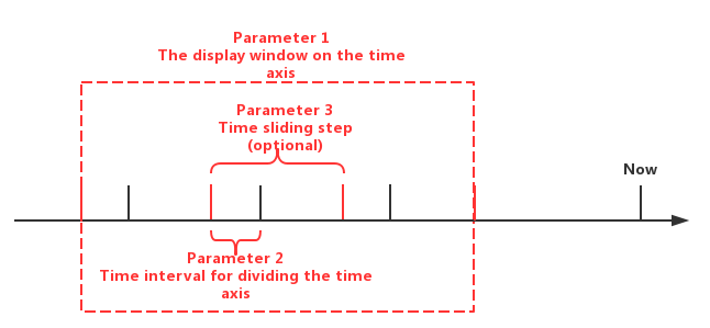
The GROUP BY statement provides users with three types of specified parameters:

Parameter 1: The display window on the time axis
Parameter 2: Time interval for dividing the time axis(should be positive)
Parameter 3: Time sliding step (optional and should not be smaller than the time interval and defaults to equal the time interval if not set)

The actual meanings of the three types of parameters are shown in Figure below.
Among them, the parameter 3 is optional.

There are three typical examples of frequency reduction aggregation:

Downsampling Aggregate Query without Specifying the Sliding Step Length

The SQL statement is:

select count(status), max_value(temperature) from root.ln.wf01.wt01 group by ([2017-11-01T00:00:00, 2017-11-07T23:00:00),1d);

which means:

Since the sliding step length is not specified, the GROUP BY statement by default set the sliding step the same as the time interval which is 1d.

The fist parameter of the GROUP BY statement above is the display window parameter, which determines the final display range is [2017-11-01T00:00:00, 2017-11-07T23:00:00).

The second parameter of the GROUP BY statement above is the time interval for dividing the time axis. Taking this parameter (1d) as time interval and startTime of the display window as the dividing origin, the time axis is divided into several continuous intervals, which are [0,1d), [1d, 2d), [2d, 3d), etc.

Then the system will use the time and value filtering condition in the WHERE clause and the first parameter of the GROUP BY statement as the data filtering condition to obtain the data satisfying the filtering condition (which in this case is the data in the range of [2017-11-01T00:00:00, 2017-11-07 T23:00:00]), and map these data to the previously segmented time axis (in this case there are mapped data in every 1-day period from 2017-11-01T00:00:00 to 2017-11-07T23:00:00:00).

Since there is data for each time period in the result range to be displayed, the execution result of the SQL statement is shown below:

+-----------------------------+-------------------------------+----------------------------------------+
|                         Time|count(root.ln.wf01.wt01.status)|max_value(root.ln.wf01.wt01.temperature)|
+-----------------------------+-------------------------------+----------------------------------------+
|2017-11-01T00:00:00.000+08:00|                           1440|                                    26.0|
|2017-11-02T00:00:00.000+08:00|                           1440|                                    26.0|
|2017-11-03T00:00:00.000+08:00|                           1440|                                   25.99|
|2017-11-04T00:00:00.000+08:00|                           1440|                                    26.0|
|2017-11-05T00:00:00.000+08:00|                           1440|                                    26.0|
|2017-11-06T00:00:00.000+08:00|                           1440|                                   25.99|
|2017-11-07T00:00:00.000+08:00|                           1380|                                    26.0|
+-----------------------------+-------------------------------+----------------------------------------+
Total line number = 7
It costs 0.024s

Downsampling Aggregate Query Specifying the Sliding Step Length

The SQL statement is:

select count(status), max_value(temperature) from root.ln.wf01.wt01 group by ([2017-11-01 00:00:00, 2017-11-07 23:00:00), 3h, 1d);

which means:

Since the user specifies the sliding step parameter as 1d, the GROUP BY statement will move the time interval 1 day long instead of 3 hours as default.

That means we want to fetch all the data of 00:00:00 to 02:59:59 every day from 2017-11-01 to 2017-11-07.

The first parameter of the GROUP BY statement above is the display window parameter, which determines the final display range is [2017-11-01T00:00:00, 2017-11-07T23:00:00).

The second parameter of the GROUP BY statement above is the time interval for dividing the time axis. Taking this parameter (3h) as time interval and the startTime of the display window as the dividing origin, the time axis is divided into several continuous intervals, which are [2017-11-01T00:00:00, 2017-11-01T03:00:00), [2017-11-02T00:00:00, 2017-11-02T03:00:00), [2017-11-03T00:00:00, 2017-11-03T03:00:00), etc.

The third parameter of the GROUP BY statement above is the sliding step for each time interval moving.

Then the system will use the time and value filtering condition in the WHERE clause and the first parameter of the GROUP BY statement as the data filtering condition to obtain the data satisfying the filtering condition (which in this case is the data in the range of [2017-11-01T00:00:00, 2017-11-07T23:00:00]), and map these data to the previously segmented time axis (in this case there are mapped data in every 3-hour period for each day from 2017-11-01T00:00:00 to 2017-11-07T23:00:00:00).

Since there is data for each time period in the result range to be displayed, the execution result of the SQL statement is shown below:

+-----------------------------+-------------------------------+----------------------------------------+
|                         Time|count(root.ln.wf01.wt01.status)|max_value(root.ln.wf01.wt01.temperature)|
+-----------------------------+-------------------------------+----------------------------------------+
|2017-11-01T00:00:00.000+08:00|                            180|                                   25.98|
|2017-11-02T00:00:00.000+08:00|                            180|                                   25.98|
|2017-11-03T00:00:00.000+08:00|                            180|                                   25.96|
|2017-11-04T00:00:00.000+08:00|                            180|                                   25.96|
|2017-11-05T00:00:00.000+08:00|                            180|                                    26.0|
|2017-11-06T00:00:00.000+08:00|                            180|                                   25.85|
|2017-11-07T00:00:00.000+08:00|                            180|                                   25.99|
+-----------------------------+-------------------------------+----------------------------------------+
Total line number = 7
It costs 0.006s

Downsampling Aggregate Query by Natural Month

The SQL statement is:

select count(status) from root.ln.wf01.wt01 group by([2017-11-01T00:00:00, 2019-11-07T23:00:00), 1mo, 2mo);

which means:

Since the user specifies the sliding step parameter as 2mo, the GROUP BY statement will move the time interval 2 months long instead of 1 month as default.

The first parameter of the GROUP BY statement above is the display window parameter, which determines the final display range is [2017-11-01T00:00:00, 2019-11-07T23:00:00).

The start time is 2017-11-01T00:00:00. The sliding step will increment monthly based on the start date, and the 1st day of the month will be used as the time interval's start time.

The second parameter of the GROUP BY statement above is the time interval for dividing the time axis. Taking this parameter (1mo) as time interval and the startTime of the display window as the dividing origin, the time axis is divided into several continuous intervals, which are [2017-11-01T00:00:00, 2017-12-01T00:00:00), [2018-02-01T00:00:00, 2018-03-01T00:00:00), [2018-05-03T00:00:00, 2018-06-01T00:00:00)), etc.

The third parameter of the GROUP BY statement above is the sliding step for each time interval moving.

Then the system will use the time and value filtering condition in the WHERE clause and the first parameter of the GROUP BY statement as the data filtering condition to obtain the data satisfying the filtering condition (which in this case is the data in the range of (2017-11-01T00:00:00, 2019-11-07T23:00:00], and map these data to the previously segmented time axis (in this case there are mapped data of the first month in every two month period from 2017-11-01T00:00:00 to 2019-11-07T23:00:00).

The SQL execution result is:

+-----------------------------+-------------------------------+
|                         Time|count(root.ln.wf01.wt01.status)|
+-----------------------------+-------------------------------+
|2017-11-01T00:00:00.000+08:00|                            259|
|2018-01-01T00:00:00.000+08:00|                            250|
|2018-03-01T00:00:00.000+08:00|                            259|
|2018-05-01T00:00:00.000+08:00|                            251|
|2018-07-01T00:00:00.000+08:00|                            242|
|2018-09-01T00:00:00.000+08:00|                            225|
|2018-11-01T00:00:00.000+08:00|                            216|
|2019-01-01T00:00:00.000+08:00|                            207|
|2019-03-01T00:00:00.000+08:00|                            216|
|2019-05-01T00:00:00.000+08:00|                            207|
|2019-07-01T00:00:00.000+08:00|                            199|
|2019-09-01T00:00:00.000+08:00|                            181|
|2019-11-01T00:00:00.000+08:00|                             60|
+-----------------------------+-------------------------------+

The SQL statement is:

select count(status) from root.ln.wf01.wt01 group by([2017-10-31T00:00:00, 2019-11-07T23:00:00), 1mo, 2mo);

which means:

Since the user specifies the sliding step parameter as 2mo, the GROUP BY statement will move the time interval 2 months long instead of 1 month as default.

The first parameter of the GROUP BY statement above is the display window parameter, which determines the final display range is [2017-10-31T00:00:00, 2019-11-07T23:00:00).

Different from the previous example, the start time is set to 2017-10-31T00:00:00. The sliding step will increment monthly based on the start date, and the 31st day of the month meaning the last day of the month will be used as the time interval's start time. If the start time is set to the 30th date, the sliding step will use the 30th or the last day of the month.

The start time is 2017-10-31T00:00:00. The sliding step will increment monthly based on the start time, and the 1st day of the month will be used as the time interval's start time.

The second parameter of the GROUP BY statement above is the time interval for dividing the time axis. Taking this parameter (1mo) as time interval and the startTime of the display window as the dividing origin, the time axis is divided into several continuous intervals, which are [2017-10-31T00:00:00, 2017-11-31T00:00:00), [2018-02-31T00:00:00, 2018-03-31T00:00:00), [2018-05-31T00:00:00, 2018-06-31T00:00:00), etc.

The third parameter of the GROUP BY statement above is the sliding step for each time interval moving.

Then the system will use the time and value filtering condition in the WHERE clause and the first parameter of the GROUP BY statement as the data filtering condition to obtain the data satisfying the filtering condition (which in this case is the data in the range of [2017-10-31T00:00:00, 2019-11-07T23:00:00) and map these data to the previously segmented time axis (in this case there are mapped data of the first month in every two month period from 2017-10-31T00:00:00 to 2019-11-07T23:00:00).

The SQL execution result is:

+-----------------------------+-------------------------------+
|                         Time|count(root.ln.wf01.wt01.status)|
+-----------------------------+-------------------------------+
|2017-10-31T00:00:00.000+08:00|                            251|
|2017-12-31T00:00:00.000+08:00|                            250|
|2018-02-28T00:00:00.000+08:00|                            259|
|2018-04-30T00:00:00.000+08:00|                            250|
|2018-06-30T00:00:00.000+08:00|                            242|
|2018-08-31T00:00:00.000+08:00|                            225|
|2018-10-31T00:00:00.000+08:00|                            216|
|2018-12-31T00:00:00.000+08:00|                            208|
|2019-02-28T00:00:00.000+08:00|                            216|
|2019-04-30T00:00:00.000+08:00|                            208|
|2019-06-30T00:00:00.000+08:00|                            199|
|2019-08-31T00:00:00.000+08:00|                            181|
|2019-10-31T00:00:00.000+08:00|                             69|
+-----------------------------+-------------------------------+

Left Open And Right Close Range

The SQL statement is:

select count(status) from root.ln.wf01.wt01 group by ((2017-11-01T00:00:00, 2017-11-07T23:00:00],1d);

In this sql, the time interval is left open and right close, so we won't include the value of timestamp 2017-11-01T00:00:00 and instead we will include the value of timestamp 2017-11-07T23:00:00.

We will get the result like following:

+-----------------------------+-------------------------------+
|                         Time|count(root.ln.wf01.wt01.status)|
+-----------------------------+-------------------------------+
|2017-11-02T00:00:00.000+08:00|                           1440|
|2017-11-03T00:00:00.000+08:00|                           1440|
|2017-11-04T00:00:00.000+08:00|                           1440|
|2017-11-05T00:00:00.000+08:00|                           1440|
|2017-11-06T00:00:00.000+08:00|                           1440|
|2017-11-07T00:00:00.000+08:00|                           1440|
|2017-11-07T23:00:00.000+08:00|                           1380|
+-----------------------------+-------------------------------+
Total line number = 7
It costs 0.004s

Downsampling Aggregate Query with Level Clause

Level could be defined to show count the number of points of each node at the given level in current Metadata Tree.

This could be used to query the number of points under each device.

The SQL statement is:

Get downsampling aggregate query by level.

select count(status) from root.ln.wf01.wt01 group by ((2017-11-01T00:00:00, 2017-11-07T23:00:00],1d), level=1;

Result:

+-----------------------------+-------------------------+
|                         Time|COUNT(root.ln.*.*.status)|
+-----------------------------+-------------------------+
|2017-11-02T00:00:00.000+08:00|                     1440|
|2017-11-03T00:00:00.000+08:00|                     1440|
|2017-11-04T00:00:00.000+08:00|                     1440|
|2017-11-05T00:00:00.000+08:00|                     1440|
|2017-11-06T00:00:00.000+08:00|                     1440|
|2017-11-07T00:00:00.000+08:00|                     1440|
|2017-11-07T23:00:00.000+08:00|                     1380|
+-----------------------------+-------------------------+
Total line number = 7
It costs 0.006s

Downsampling aggregate query with sliding step and by level.

select count(status) from root.ln.wf01.wt01 group by ([2017-11-01 00:00:00, 2017-11-07 23:00:00), 3h, 1d), level=1;

Result:

+-----------------------------+-------------------------+
|                         Time|COUNT(root.ln.*.*.status)|
+-----------------------------+-------------------------+
|2017-11-01T00:00:00.000+08:00|                      180|
|2017-11-02T00:00:00.000+08:00|                      180|
|2017-11-03T00:00:00.000+08:00|                      180|
|2017-11-04T00:00:00.000+08:00|                      180|
|2017-11-05T00:00:00.000+08:00|                      180|
|2017-11-06T00:00:00.000+08:00|                      180|
|2017-11-07T00:00:00.000+08:00|                      180|
+-----------------------------+-------------------------+
Total line number = 7
It costs 0.004s