AINode
AINode
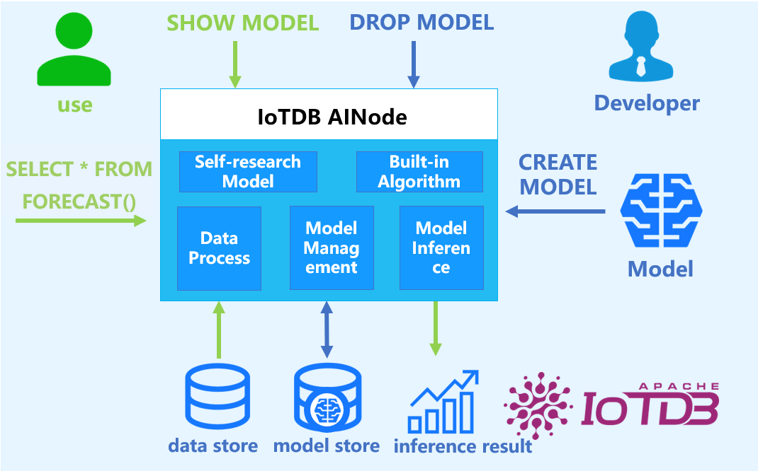
AINode is a native IoTDB node that supports the registration, management, and invocation of time-series-related models. It comes with built-in industry-leading self-developed time-series large models, such as the Timer series developed by Tsinghua University. These models can be invoked through standard SQL statements, enabling real-time inference of time series data at the millisecond level, and supporting application scenarios such as trend forecasting, missing value imputation, and anomaly detection for time series data.
Available since V2.0.5
The system architecture is shown below:
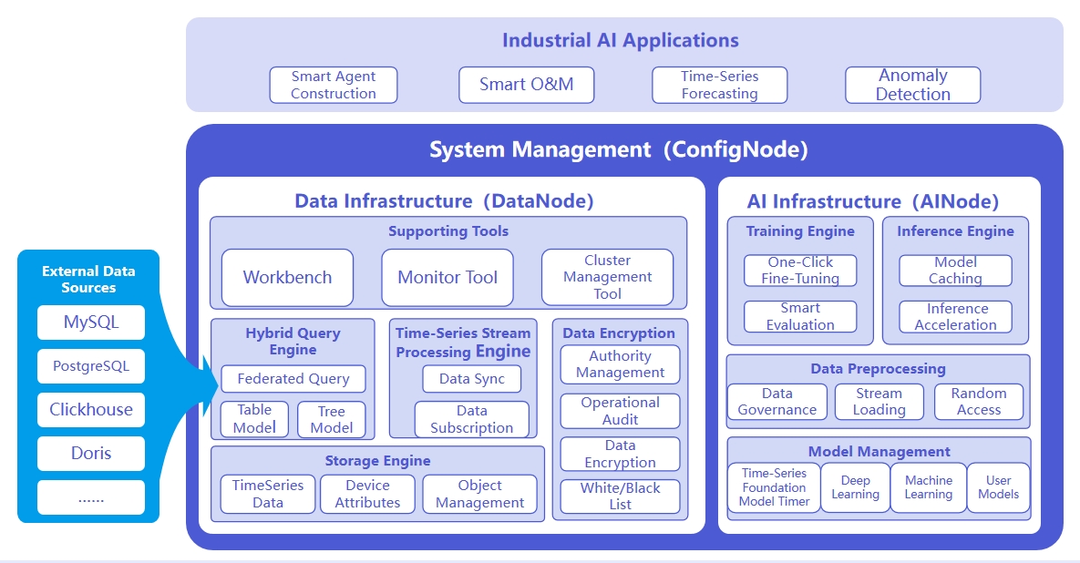
The responsibilities of the three nodes are as follows:
- ConfigNode:
- Manages distributed nodes and handles load balancing across the system.
- DataNode:
- Receives and parses user SQL queries.
- Stores time-series data.
- Performs preprocessing computations on raw data.
- AINode:
- Manages and utilizes time-series models (including training/inference).
- Supports deep learning and machine learning workflows.
1. Advantageous features
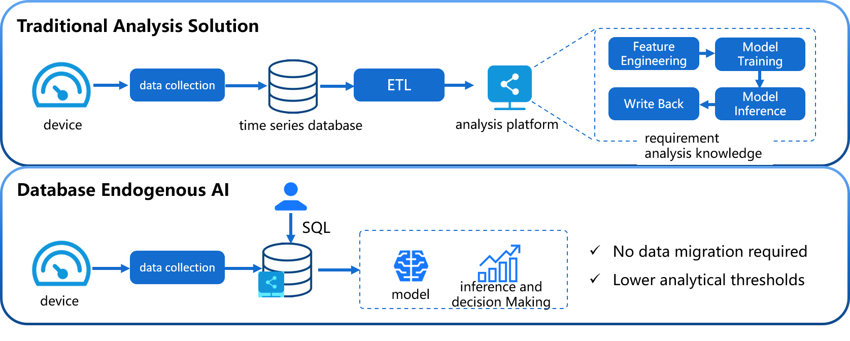
Compared with building a machine learning service alone, it has the following advantages:
Simple and easy to use: no need to use Python or Java programming, the complete process of machine learning model management and inference can be completed using SQL statements. Creating a model can be done using the CREATE MODEL statement, and using a model for inference can be done using the CALL INFERENCE (...) statement, making it simpler and more convenient to use.
Avoid Data Migration: With IoTDB native machine learning, data stored in IoTDB can be directly applied to the inference of machine learning models without having to move the data to a separate machine learning service platform, which accelerates data processing, improves security, and reduces costs.
- Built-in Advanced Algorithms: supports industry-leading machine learning analytics algorithms covering typical timing analysis tasks, empowering the timing database with native data analysis capabilities. Such as:
- Time Series Forecasting: learns patterns of change from past time series; thus outputs the most likely prediction of future series based on observations at a given past time.
- Anomaly Detection for Time Series: detects and identifies outliers in a given time series data, helping to discover anomalous behaviour in the time series.
- Annotation for Time Series (Time Series Annotation): Adds additional information or markers, such as event occurrence, outliers, trend changes, etc., to each data point or specific time period to better understand and analyse the data.
2. Basic Concepts
- Model: A machine learning model that takes time series data as input and outputs analysis results or decisions. Models are the basic management units of AINode, supporting model operations such as creation (registration), deletion, query, and inference.
- Create: Load externally designed or trained model files or algorithms into MLNode for unified management and use by IoTDB.
- Inference: The process of using the created model to complete the timing analysis task applicable to the model on the specified timing data.
- Built-in capabilities: AINode comes with machine learning algorithms or home-grown models for common timing analysis scenarios (e.g., prediction and anomaly detection).
3. Installation and Deployment
The deployment of AINode can be found in the document AINode Deployment.
4. Usage Guidelines
AINode provides model creation and deletion functions for time series models. Built-in models do not require creation and can be used directly.
4.1 Registering Models
Trained deep learning models can be registered by specifying their input and output vector dimensions for inference.
Models that meet the following criteria can be registered with AINode:
- AINode currently supports models trained with PyTorch 2.4.0. Features above version 2.4.0 should be avoided.
- AINode supports models stored using PyTorch JIT (
model.pt), which must include both the model structure and weights. - The model input sequence can include single or multiple columns. If multi-column, it must match the model capabilities and configuration file.
- Model configuration parameters must be clearly defined in the
config.yamlfile. When using the model, the input and output dimensions defined inconfig.yamlmust be strictly followed. Mismatches with the configuration file will cause errors.
The SQL syntax for model registration is defined as follows:
create model <model_id> using uri <uri>Detailed meanings of SQL parameters:
model_id: The global unique identifier for the model, non-repeating. Model names have the following constraints:
- Allowed characters: [0-9 a-z A-Z _] (letters, digits (not at the beginning), underscores (not at the beginning))
- Length: 2-64 characters
- Case-sensitive
uri: The resource path of the model registration files, which should include the model structure and weight file
model.ptand the model configuration fileconfig.yamlModel structure and weight file: The weight file generated after model training, currently supporting
.ptfiles from PyTorch training.Model configuration file: Parameters related to the model structure provided during registration, which must include input and output dimensions for inference:
Parameter Name Description Example input_shape Rows and columns of model input [96,2] output_shape Rows and columns of model output [48,2] In addition to inference, data types of input and output can also be specified:
Parameter Name Description Example input_type Data type of model input ['float32', 'float32'] output_type Data type of model output ['float32', 'float32'] Additional notes can be specified for model management display:
Parameter Name Description Example attributes Optional notes set by users for model display 'model_type': 'dlinear', 'kernel_size': '25'
In addition to registering local model files, remote resource paths can be specified via URIs for registration, using open-source model repositories (e.g., HuggingFace).
Example
The example folder contains model.pt (trained model) and config.yaml with the following content:
configs:
    # Required
    input_shape: [96, 2]      # Model accepts 96 rows x 2 columns of data
    output_shape: [48, 2]     # Model outputs 48 rows x 2 columns of data

    # Optional (default to all float32, column count matches shape)
    input_type: ["int64", "int64"]  # Data types of inputs, must match input column count
    output_type: ["text", "int64"]  # Data types of outputs, must match output column count

attributes:           # Optional user-defined notes
   'model_type': 'dlinear'
   'kernel_size': '25'
Register the model by specifying this folder as the loading path:
IoTDB> create model dlinear_example using uri "file://./example"After SQL execution, registration proceeds asynchronously. The registration status can be checked via model display (see Model Display section). The registration success time mainly depends on the model file size.
Once registered, the model can be invoked for inference through normal query syntax.
4.2 Viewing Models
Successfully registered models can be queried for model-specific information through the show models command. The SQL definition is as follows:
show models

show models <model_id>
In addition to displaying all models, specifying a model_id shows details of a specific model. The display includes:
| ModelId | ModelType | Category | State |
|---|---|---|---|
| Model ID | Model Type | Model Category | Model State |
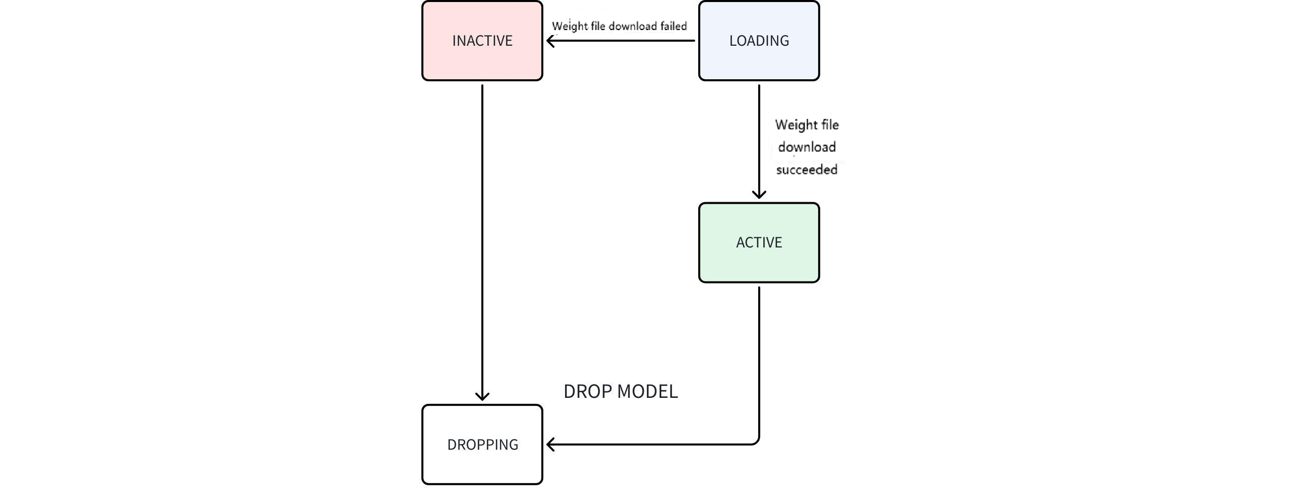
- Model State Transition Diagram
Instructions:
- Initialization:
- When AINode starts, show models only displays BUILT-IN models.
- Custom Model Import:
- Users can import custom models (marked as USER-DEFINED).
- The system attempts to parse the ModelTypefrom the config file.
- If parsing fails, the field remains empty.
- Foundation Model Weights:
- Time-series foundation model weights are not bundled with AINode.
- AINode automatically downloads them during startup.
- Download state: LOADING.
- Download Outcomes:
- Success → State changes to ACTIVE.
- Failure → State changes to INACTIVE.
Example
IoTDB> show models
+---------------------+--------------------+--------------+---------+
|              ModelId|           ModelType|      Category|    State|
+---------------------+--------------------+--------------+---------+
|                arima|               Arima|      BUILT-IN|   ACTIVE|
|          holtwinters|         HoltWinters|      BUILT-IN|   ACTIVE|
|exponential_smoothing|ExponentialSmoothing|      BUILT-IN|   ACTIVE|
|     naive_forecaster|     NaiveForecaster|      BUILT-IN|   ACTIVE|
|       stl_forecaster|       StlForecaster|      BUILT-IN|   ACTIVE|
|         gaussian_hmm|         GaussianHmm|      BUILT-IN|   ACTIVE|
|              gmm_hmm|              GmmHmm|      BUILT-IN|   ACTIVE|
|                stray|               Stray|      BUILT-IN|   ACTIVE|
|               custom|                    |  USER-DEFINED|   ACTIVE|
|             timer_xl|            Timer-XL|      BUILT-IN|  LOADING|
|              sundial|       Timer-Sundial|      BUILT-IN|   ACTIVE|
+---------------------+--------------------+--------------+---------+
4.3 Deleting Models
Registered models can be deleted via SQL, which removes all related files under AINode:
drop model <model_id>Specify the registered model_id to delete the model. Since deletion involves data cleanup, the operation is not immediate, and the model state becomes DROPPING, during which it cannot be used for inference. Note: Built-in models cannot be deleted.
4.4 Using Built-in Model Reasoning
SQL syntax:
call inference(<model_id>,inputSql,(<parameterName>=<parameterValue>)*)

window_function:
    head(window_size)
    tail(window_size)
    count(window_size,sliding_step)
Built-in model inference does not require a registration process, the inference function can be used by calling the inference function through the call keyword, and its corresponding parameters are described as follows:
built_in_model_name: built-in model name
parameterName: parameter name
parameterValue: parameter value
Note: To use a built-in time series large model for inference, the corresponding model weights must be stored locally in the directory
/IOTDB_AINODE_HOME/data/ainode/models/weights/model_id/. If the weights are not present locally, they will be automatically downloaded from HuggingFace. Ensure your environment has direct access to HuggingFace.
Built-in Models and Parameter Descriptions
The following machine learning models are currently built-in, please refer to the following links for detailed parameter descriptions.
| Model | built_in_model_name | Task type | Parameter description |
|---|---|---|---|
| Arima | _Arima | Forecast | Arima Parameter description |
| STLForecaster | _STLForecaster | Forecast | STLForecaster Parameter description |
| NaiveForecaster | _NaiveForecaster | Forecast | NaiveForecaster Parameter description |
| ExponentialSmoothing | _ExponentialSmoothing | Forecast | ExponentialSmoothing Parameter description |
| GaussianHMM | _GaussianHMM | Annotation | GaussianHMMParameter description |
| GMMHMM | _GMMHMM | Annotation | GMMHMM Parameter description |
| Stray | _Stray | Anomaly detection | Stray Parameter description |
After completing the registration of the model, the inference function can be used by calling the inference function through the call keyword, and its corresponding parameters are described as follows:
- model_id: corresponds to a registered model
- sql: sql query statement, the result of the query is used as input to the model for model inference. The dimensions of the rows and columns in the result of the query need to match the size specified in the specific model config. (It is not recommended to use the
SELECT *clause for the sql here because in IoTDB,*does not sort the columns, so the order of the columns is undefined, you can useSELECT s0,s1to ensure that the columns order matches the expectations of the model input) - window_function: Window functions that can be used in the inference process, there are currently three types of window functions provided to assist in model inference:
head(window_size): Get the top window_size points in the data for model inference, this window can be used for data cropping.
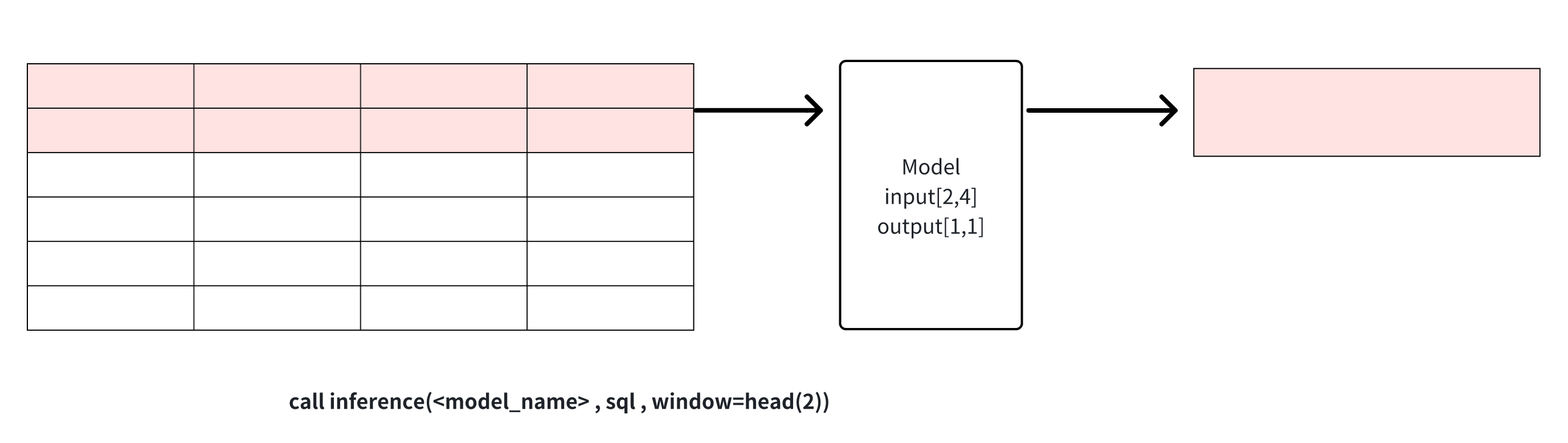
tail(window_size): get the last window_size point in the data for model inference, this window can be used for data cropping.
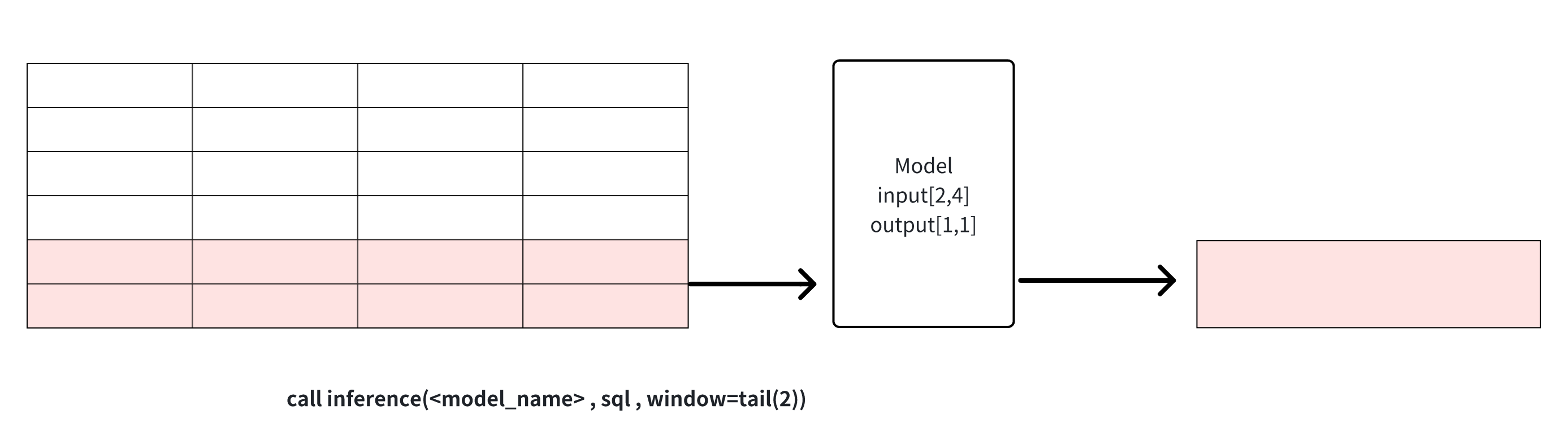
count(window_size, sliding_step): sliding window based on the number of points, the data in each window will be reasoned through the model respectively, as shown in the example below, window_size for 2 window function will be divided into three windows of the input dataset, and each window will perform reasoning operations to generate results respectively. The window can be used for continuous inference

Explanation 1: window can be used to solve the problem of cropping rows when the results of the sql query and the input row requirements of the model do not match. Note that when the number of columns does not match or the number of rows is directly less than the model requirement, the inference cannot proceed and an error message will be returned.
Explanation 2: In deep learning applications, timestamp-derived features (time columns in the data) are often used as covariates in generative tasks, and are input into the model together to enhance the model, but the time columns are generally not included in the model's output. In order to ensure the generality of the implementation, the model inference results only correspond to the real output of the model, if the model does not output the time column, it will not be included in the results.
Example
The following is an example of inference in action using a deep learning model, for the dlinear prediction model with input [96,2] and output [48,2] mentioned above, which we use via SQL.
IoTDB> select s1,s2 from root.**
+-----------------------------+-------------------+-------------------+
|                         Time|    root.eg.etth.s0|    root.eg.etth.s1|
+-----------------------------+-------------------+-------------------+
|1990-01-01T00:00:00.000+08:00|             0.7855|              1.611|
|1990-01-02T00:00:00.000+08:00|             0.7818|               1.61|
|1990-01-03T00:00:00.000+08:00|             0.7867|             1.6293|
|1990-01-04T00:00:00.000+08:00|              0.786|              1.637|
|1990-01-05T00:00:00.000+08:00|             0.7849|              1.653|
|1990-01-06T00:00:00.000+08:00|             0.7866|             1.6537|
|1990-01-07T00:00:00.000+08:00|             0.7886|              1.662|
......
|1990-03-31T00:00:00.000+08:00|             0.7585|              1.678|
|1990-04-01T00:00:00.000+08:00|             0.7587|             1.6763|
|1990-04-02T00:00:00.000+08:00|               0.76|             1.6813|
|1990-04-03T00:00:00.000+08:00|             0.7669|              1.684|
|1990-04-04T00:00:00.000+08:00|             0.7645|              1.677|
|1990-04-05T00:00:00.000+08:00|             0.7625|               1.68|
|1990-04-06T00:00:00.000+08:00|             0.7617|             1.6917|
+-----------------------------+-------------------+-------------------+
Total line number = 96

IoTDB> call inference(dlinear_example,"select s0,s1 from root.**", generateTime=True)
+-----------------------------+--------------------------------------------+-----------------------------+
|                         Time|                                   _result_0|                    _result_1|
+-----------------------------+--------------------------------------------+-----------------------------+
|1990-04-06T00:00:00.000+08:00|                           0.726302981376648|           1.6549958229064941|
|1990-04-08T00:00:00.000+08:00|                          0.7354921698570251|           1.6482787370681763|
|1990-04-10T00:00:00.000+08:00|                          0.7238251566886902|           1.6278168201446533|
......
|1990-07-07T00:00:00.000+08:00|                          0.7692174911499023|            1.654654049873352|
|1990-07-09T00:00:00.000+08:00|                          0.7685555815696716|           1.6625318765640259|
|1990-07-11T00:00:00.000+08:00|                          0.7856493592262268|           1.6508299350738525|
+-----------------------------+--------------------------------------------+-----------------------------+
Total line number = 48
Example of using the tail/head window function
When the amount of data is variable and you want to take the latest 96 rows of data for inference, you can use the corresponding window function tail. head function is used in a similar way, except that it takes the earliest 96 points.
IoTDB> select s1,s2 from root.**
+-----------------------------+-------------------+-------------------+
|                         Time|    root.eg.etth.s0|    root.eg.etth.s1|
+-----------------------------+-------------------+-------------------+
|1988-01-01T00:00:00.000+08:00|             0.7355|              1.211|
......
|1990-01-01T00:00:00.000+08:00|             0.7855|              1.611|
|1990-01-02T00:00:00.000+08:00|             0.7818|               1.61|
|1990-01-03T00:00:00.000+08:00|             0.7867|             1.6293|
|1990-01-04T00:00:00.000+08:00|              0.786|              1.637|
|1990-01-05T00:00:00.000+08:00|             0.7849|              1.653|
|1990-01-06T00:00:00.000+08:00|             0.7866|             1.6537|
|1990-01-07T00:00:00.000+08:00|             0.7886|              1.662|
......
|1990-03-31T00:00:00.000+08:00|             0.7585|              1.678|
|1990-04-01T00:00:00.000+08:00|             0.7587|             1.6763|
|1990-04-02T00:00:00.000+08:00|               0.76|             1.6813|
|1990-04-03T00:00:00.000+08:00|             0.7669|              1.684|
|1990-04-04T00:00:00.000+08:00|             0.7645|              1.677|
|1990-04-05T00:00:00.000+08:00|             0.7625|               1.68|
|1990-04-06T00:00:00.000+08:00|             0.7617|             1.6917|
+-----------------------------+-------------------+-------------------+
Total line number = 996

IoTDB> call inference(dlinear_example,"select s0,s1 from root.**", generateTime=True, window=tail(96))
+-----------------------------+--------------------------------------------+-----------------------------+
|                         Time|                                   _result_0|                    _result_1|
+-----------------------------+--------------------------------------------+-----------------------------+
|1990-04-06T00:00:00.000+08:00|                           0.726302981376648|           1.6549958229064941|
|1990-04-08T00:00:00.000+08:00|                          0.7354921698570251|           1.6482787370681763|
|1990-04-10T00:00:00.000+08:00|                          0.7238251566886902|           1.6278168201446533|
......
|1990-07-07T00:00:00.000+08:00|                          0.7692174911499023|            1.654654049873352|
|1990-07-09T00:00:00.000+08:00|                          0.7685555815696716|           1.6625318765640259|
|1990-07-11T00:00:00.000+08:00|                          0.7856493592262268|           1.6508299350738525|
+-----------------------------+--------------------------------------------+-----------------------------+
Total line number = 48
Example of using the count window function
This window is mainly used for computational tasks. When the task's corresponding model can only handle a fixed number of rows of data at a time, but the final desired outcome is multiple sets of prediction results, this window function can be used to perform continuous inference using a sliding window of points. Suppose we now have an anomaly detection model anomaly_example(input: [24,2], output[1,1]), which generates a 0/1 label for every 24 rows of data. An example of its use is as follows:
IoTDB> select s1,s2 from root.**
+-----------------------------+-------------------+-------------------+
|                         Time|    root.eg.etth.s0|    root.eg.etth.s1|
+-----------------------------+-------------------+-------------------+
|1990-01-01T00:00:00.000+08:00|             0.7855|              1.611|
|1990-01-02T00:00:00.000+08:00|             0.7818|               1.61|
|1990-01-03T00:00:00.000+08:00|             0.7867|             1.6293|
|1990-01-04T00:00:00.000+08:00|              0.786|              1.637|
|1990-01-05T00:00:00.000+08:00|             0.7849|              1.653|
|1990-01-06T00:00:00.000+08:00|             0.7866|             1.6537|
|1990-01-07T00:00:00.000+08:00|             0.7886|              1.662|
......
|1990-03-31T00:00:00.000+08:00|             0.7585|              1.678|
|1990-04-01T00:00:00.000+08:00|             0.7587|             1.6763|
|1990-04-02T00:00:00.000+08:00|               0.76|             1.6813|
|1990-04-03T00:00:00.000+08:00|             0.7669|              1.684|
|1990-04-04T00:00:00.000+08:00|             0.7645|              1.677|
|1990-04-05T00:00:00.000+08:00|             0.7625|               1.68|
|1990-04-06T00:00:00.000+08:00|             0.7617|             1.6917|
+-----------------------------+-------------------+-------------------+
Total line number = 96

IoTDB> call inference(anomaly_example,"select s0,s1 from root.**", generateTime=True, window=count(24,24))
+-----------------------------+-------------------------+
|                         Time|                _result_0|
+-----------------------------+-------------------------+
|1990-04-06T00:00:00.000+08:00|                        0|
|1990-04-30T00:00:00.000+08:00|                        1|
|1990-05-24T00:00:00.000+08:00|                        1|
|1990-06-17T00:00:00.000+08:00|                        0|
+-----------------------------+-------------------------+
Total line number = 4
In the result set, each row's label corresponds to the output of the anomaly detection model after inputting each group of 24 rows of data.
4.5 Time Series Large Model Import Steps
AINode supports multiple time series large models. For deployment, refer to Time Series Large Model
5. Privilege Management
When using AINode related functions, the authentication of IoTDB itself can be used to do a permission management, users can only use the model management related functions when they have the USE_MODEL permission. When using the inference function, the user needs to have the permission to access the source sequence corresponding to the SQL of the input model.
| Privilege Name | Privilege Scope | Administrator User (default ROOT) | Normal User | Path Related |
|---|---|---|---|---|
| USE_MODEL | create model/show models/drop model | √ | √ | x |
| READ_DATA | call inference | √ | √ | √ |
6. Practical Examples
6.1 Power Load Prediction
In some industrial scenarios, there is a need to predict power loads, which can be used to optimise power supply, conserve energy and resources, support planning and expansion, and enhance power system reliability.
The data for the test set of ETTh1 that we use is ETTh1.
It contains power data collected at 1h intervals, and each data consists of load and oil temperature as High UseFul Load, High UseLess Load, Middle UseLess Load, Low UseFul Load, Low UseLess Load, Oil Temperature.
On this dataset, the model inference function of IoTDB-ML can predict the oil temperature in the future period of time through the relationship between the past values of high, middle and low use loads and the corresponding time stamp oil temperature, which empowers the automatic regulation and monitoring of grid transformers.
Step 1: Data Import
Users can import the ETT dataset into IoTDB using import-data.sh in the tools folder
Bash bash ./import-data.sh -ft csv -h 127.0.0.1 -p 6667 -u root -pw root -s /path/ETTh1.csv
Step 2: Model Import
We can enter the following SQL in iotdb-cli to pull a trained model from huggingface for registration for subsequent inference.
create model dlinear using uri 'https://huggingface.co/hvlgo/dlinear/tree/main'This model is trained on the lighter weight deep model DLinear, which is able to capture as many trends within a sequence and relationships between variables as possible with relatively fast inference, making it more suitable for fast real-time prediction than other deeper models.
Step 3: Model inference
IoTDB> select s0,s1,s2,s3,s4,s5,s6 from root.eg.etth LIMIT 96
+-----------------------------+---------------+---------------+---------------+---------------+---------------+---------------+---------------+
|                         Time|root.eg.etth.s0|root.eg.etth.s1|root.eg.etth.s2|root.eg.etth.s3|root.eg.etth.s4|root.eg.etth.s5|root.eg.etth.s6|
+-----------------------------+---------------+---------------+---------------+---------------+---------------+---------------+---------------+
|2017-10-20T00:00:00.000+08:00|         10.449|          3.885|          8.706|          2.025|          2.041|          0.944|          8.864|
|2017-10-20T01:00:00.000+08:00|         11.119|          3.952|          8.813|           2.31|          2.071|          1.005|          8.442|
|2017-10-20T02:00:00.000+08:00|          9.511|           2.88|          7.533|          1.564|          1.949|          0.883|           8.16|
|2017-10-20T03:00:00.000+08:00|          9.645|           2.21|          7.249|          1.066|          1.828|          0.914|          7.949|
......
|2017-10-23T20:00:00.000+08:00|          8.105|          0.938|          4.371|         -0.569|          3.533|          1.279|          9.708|
|2017-10-23T21:00:00.000+08:00|          7.167|          1.206|          4.087|         -0.462|          3.107|          1.432|          8.723|
|2017-10-23T22:00:00.000+08:00|            7.1|           1.34|          4.015|          -0.32|          2.772|           1.31|          8.864|
|2017-10-23T23:00:00.000+08:00|          9.176|          2.746|          7.107|          1.635|           2.65|          1.097|          9.004|
+-----------------------------+---------------+---------------+---------------+---------------+---------------+---------------+---------------+
Total line number = 96

IoTDB> call inference(dlinear_example, "select s0,s1,s2,s3,s4,s5,s6 from root.eg.etth", generateTime=True, window=head(96))
+-----------------------------+-----------+----------+----------+------------+---------+----------+----------+
|                         Time|    output0|   output1|   output2|     output3|  output4|   output5|   output6|
+-----------------------------+-----------+----------+----------+------------+---------+----------+----------+
|2017-10-23T23:00:00.000+08:00|  10.319546| 3.1450553|  7.877341|   1.5723765|2.7303758| 1.1362307|  8.867775|
|2017-10-24T01:00:00.000+08:00|  10.443649| 3.3286757| 7.8593454|   1.7675098| 2.560634| 1.1177158|  8.920919|
|2017-10-24T03:00:00.000+08:00|  10.883752| 3.2341104|   8.47036|   1.6116762|2.4874182| 1.1760603|  8.798939|
......
|2017-10-26T19:00:00.000+08:00|  8.0115595| 1.2995274| 6.9900327|-0.098746896|  3.04923|  1.176214|  9.548782|
|2017-10-26T21:00:00.000+08:00|   8.612427| 2.5036244| 5.6790237|  0.66474205|2.8870275| 1.2051733|  9.330128|
|2017-10-26T22:00:00.000+08:00|  10.096699|  3.399722|    6.9909|   1.7478468|2.7642853| 1.1119363|  9.541455|
+-----------------------------+-----------+----------+----------+------------+---------+----------+----------+
Total line number = 48
We compare the results of the prediction of the oil temperature with the real results, and we can get the following image.
The data before 10/24 00:00 represents the past data input to the model, the blue line after 10/24 00:00 is the oil temperature forecast result given by the model, and the red line is the actual oil temperature data from the dataset (used for comparison).
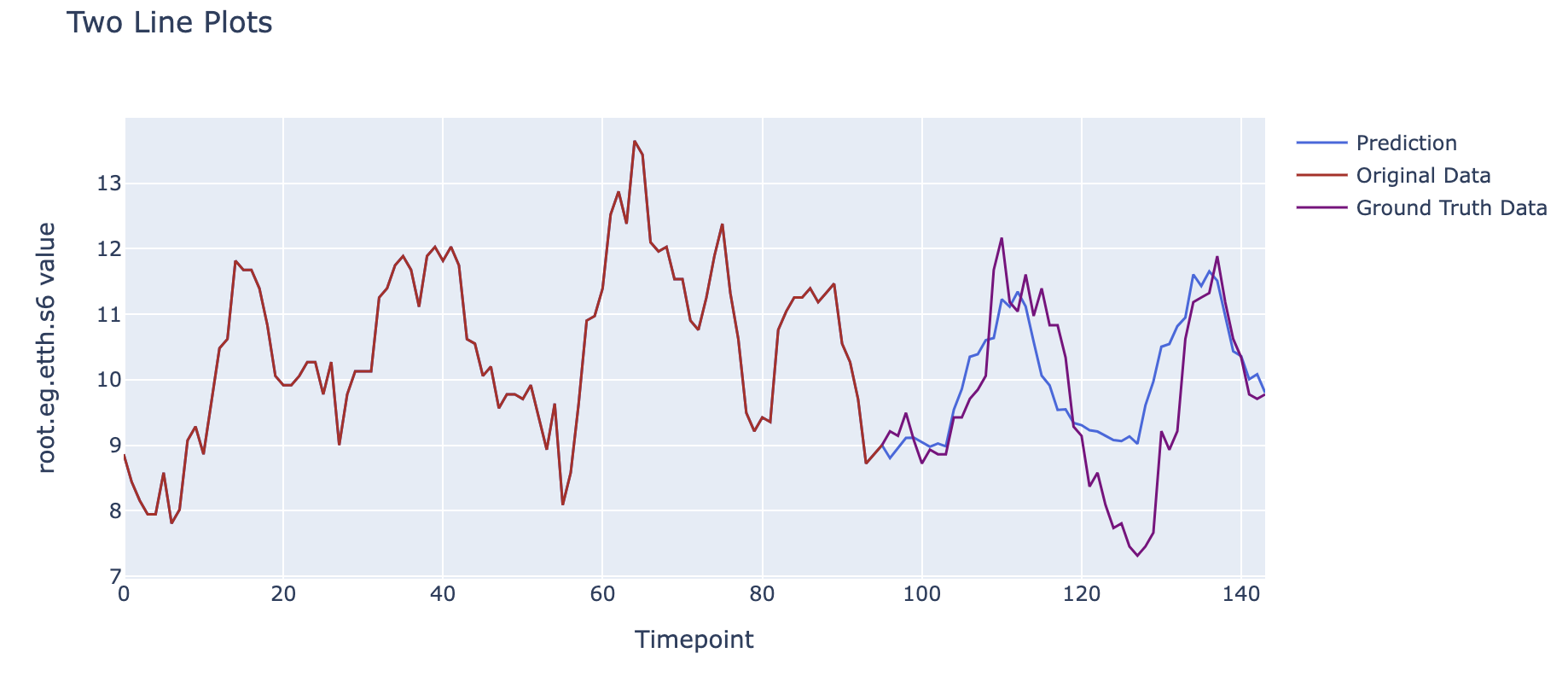
As can be seen, we have used the relationship between the six load information and the corresponding time oil temperatures for the past 96 hours (4 days) to model the possible changes in this data for the oil temperature for the next 48 hours (2 days) based on the inter-relationships between the sequences learned previously, and it can be seen that the predicted curves maintain a high degree of consistency in trend with the actual results after visualisation.
6.2 Power Prediction
Power monitoring of current, voltage and power data is required in substations for detecting potential grid problems, identifying faults in the power system, effectively managing grid loads and analysing power system performance and trends.
We have used the current, voltage and power data in a substation to form a dataset in a real scenario. The dataset consists of data such as A-phase voltage, B-phase voltage, and C-phase voltage collected every 5 - 6s for a time span of nearly four months in the substation.
The test set data content is data.
On this dataset, the model inference function of IoTDB-ML can predict the C-phase voltage in the future period through the previous values and corresponding timestamps of A-phase voltage, B-phase voltage and C-phase voltage, empowering the monitoring management of the substation.
Step 1: Data Import
Users can import the dataset using import-data.sh in the tools folder
bash ./import-data.sh -ft csv -h 127.0.0.1 -p 6667 -u root -pw root -s /path/data.csvStep 2: Model Import
We can select built-in models or registered models in IoTDB CLI for subsequent inference.
We use the built-in model STLForecaster for prediction. STLForecaster is a time series forecasting method based on the STL implementation in the statsmodels library.
Step 3: Model Inference
IoTDB> select * from root.eg.voltage limit 96
+-----------------------------+------------------+------------------+------------------+
|                         Time|root.eg.voltage.s0|root.eg.voltage.s1|root.eg.voltage.s2|
+-----------------------------+------------------+------------------+------------------+
|2023-02-14T20:38:32.000+08:00|            2038.0|            2028.0|            2041.0|
|2023-02-14T20:38:38.000+08:00|            2014.0|            2005.0|            2018.0|
|2023-02-14T20:38:44.000+08:00|            2014.0|            2005.0|            2018.0|
......
|2023-02-14T20:47:52.000+08:00|            2024.0|            2016.0|            2027.0|
|2023-02-14T20:47:57.000+08:00|            2024.0|            2016.0|            2027.0|
|2023-02-14T20:48:03.000+08:00|            2024.0|            2016.0|            2027.0|
+-----------------------------+------------------+------------------+------------------+
Total line number = 96

IoTDB> call inference(_STLForecaster, "select s0,s1,s2 from root.eg.voltage", generateTime=True, window=head(96),predict_length=48)
+-----------------------------+---------+---------+---------+
|                         Time|  output0|  output1|  output2|
+-----------------------------+---------+---------+---------+
|2023-02-14T20:48:03.000+08:00|2026.3601|2018.2953|2029.4257|
|2023-02-14T20:48:09.000+08:00|2019.1538|2011.4361|2022.0888|
|2023-02-14T20:48:15.000+08:00|2025.5074|2017.4522|2028.5199|
......

|2023-02-14T20:52:15.000+08:00|2022.2336|2015.0290|2025.1023|
|2023-02-14T20:52:21.000+08:00|2015.7241|2008.8975|2018.5085|
|2023-02-14T20:52:27.000+08:00|2022.0777|2014.9136|2024.9396|
|2023-02-14T20:52:33.000+08:00|2015.5682|2008.7821|2018.3458|
+-----------------------------+---------+---------+---------+
Total line number = 48
Comparing the predicted results of the C-phase voltage with the real results, we can get the following image.
The data before 02/14 20:48 represents the past data input to the model, the blue line after 02/14 20:48 is the predicted result of phase C voltage given by the model, while the red line is the actual phase C voltage data from the dataset (used for comparison).
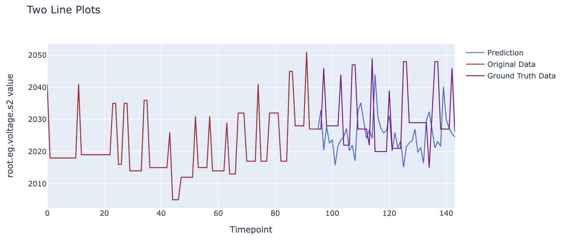
It can be seen that we used the voltage data from the past 10 minutes and, based on the previously learned inter-sequence relationships, modeled the possible changes in the phase C voltage data for the next 5 minutes. The visualized forecast curve shows a certain degree of synchronicity with the actual results in terms of trend.
6.3 Anomaly Detection
In the civil aviation and transport industry, there exists a need for anomaly detection of the number of passengers travelling on an aircraft. The results of anomaly detection can be used to guide the adjustment of flight scheduling to make the organisation more efficient.
Airline Passengers is a time-series dataset that records the number of international air passengers between 1949 and 1960, sampled at one-month intervals. The dataset contains a total of one time series. The dataset is airline.
On this dataset, the model inference function of IoTDB-ML can empower the transport industry by capturing the changing patterns of the sequence in order to detect anomalies at the sequence time points.
Step 1: Data Import
Users can import the dataset using import-data.sh in the tools folder
Bash bash ./import-data.sh -ft csv -h 127.0.0.1 -p 6667 -u root -pw root -s /path/data.csv
Step 2: Model Inference
IoTDB has some built-in machine learning algorithms that can be used directly, a sample prediction using one of the anomaly detection algorithms is shown below:
IoTDB> select * from root.eg.airline
+-----------------------------+------------------+
|                         Time|root.eg.airline.s0|
+-----------------------------+------------------+
|1949-01-31T00:00:00.000+08:00|             224.0|
|1949-02-28T00:00:00.000+08:00|             118.0|
|1949-03-31T00:00:00.000+08:00|             132.0|
|1949-04-30T00:00:00.000+08:00|             129.0|
......
|1960-09-30T00:00:00.000+08:00|             508.0|
|1960-10-31T00:00:00.000+08:00|             461.0|
|1960-11-30T00:00:00.000+08:00|             390.0|
|1960-12-31T00:00:00.000+08:00|             432.0|
+-----------------------------+------------------+
Total line number = 144

IoTDB> call inference(_Stray, "select s0 from root.eg.airline", generateTime=True, k=2)
+-----------------------------+-------+
|                         Time|output0|
+-----------------------------+-------+
|1960-12-31T00:00:00.000+08:00|      0|
|1961-01-31T08:00:00.000+08:00|      0|
|1961-02-28T08:00:00.000+08:00|      0|
|1961-03-31T08:00:00.000+08:00|      0|
......
|1972-06-30T08:00:00.000+08:00|      1|
|1972-07-31T08:00:00.000+08:00|      1|
|1972-08-31T08:00:00.000+08:00|      0|
|1972-09-30T08:00:00.000+08:00|      0|
|1972-10-31T08:00:00.000+08:00|      0|
|1972-11-30T08:00:00.000+08:00|      0|
+-----------------------------+-------+
Total line number = 144
We plot the results detected as anomalies to get the following image. Where the blue curve is the original time series and the time points specially marked with red dots are the time points that the algorithm detects as anomalies.
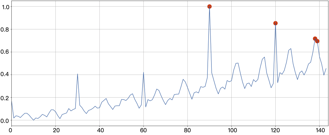
It can be seen that the Stray model has modelled the input sequence changes and successfully detected the time points where anomalies occur.